3. Part 2: Programming the PENCIL CODE

All developers are supposed to have an up-to-date entry in the pencil-code/license/developers.txt so that they can be contacted in case a code change breaks an auto-test or other code functionality.

Several Pencil Code committers have done several hundred check-ins, but many of the currently 92 registered people on the repository have hardly done anything. To put a number to this, one can define an \(h\) index, which gives the number of users who have done at least as many as that number of check-ins. This \(h\) index is currently 37, i.e., 37 users have done at least 37 check-ins; see Fig. 3.1 from 2017, when the \(h\) index was only 32.

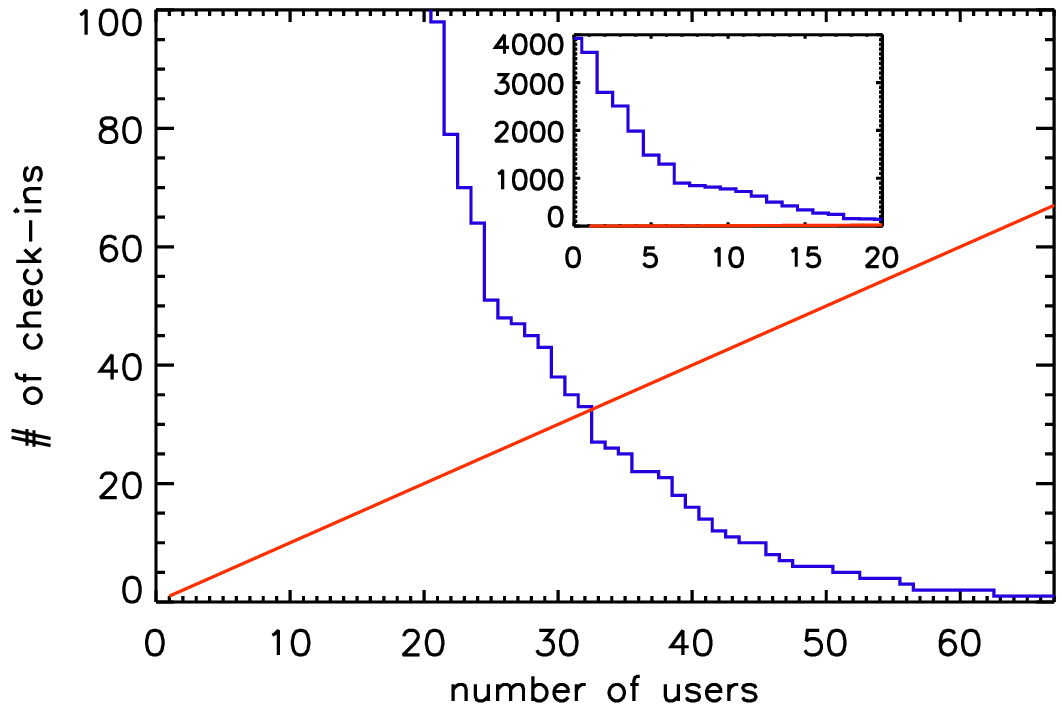
Fig. 3.1 The \(h\) index of Pencil Code check-ins in 2017.

The Pencil Code has expanded approximately linearly in the number of lines of code and the number of subroutines (Fig. 3.2). The increase in the functionality of the code is documented by the rise in the number of sample problems (Fig. 3.3). It is important to monitor the performance of the code as well. Fig. 3.4 shows that for most of the runs the run time has not changed much.

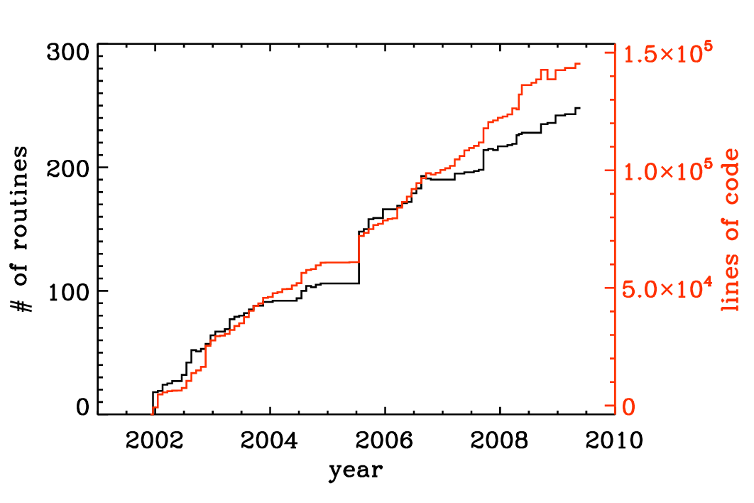
Fig. 3.2 Number of lines of code and the number of subroutines since the end of 2001. The jump in the Summer of 2005 was the moment when the developments on the side branch (eos branch) were merged with the main trunk of the code. Note the approximately linear scaling with time.

Fig. 3.3 Number of tests in the sample directory that are used in the nightly auto tests. Note again the approximately linear scaling with time.

Before making changes to the code, it is important that you verify that you can run the pc_auto-test successfully. Don’t do this when you have already modified the code, because then you cannot be sure that any problems are caused by your changes, or because it wouldn’t have worked anyway. Also, keep in mind that the code is public, so your changes should make sense from a broader perspective and should not only be intended for yourself. Regarding more general aspects about coding standards see Fortran Code.

Fig. 3.4 Run time of the daily auto-tests since August 17, 2008. For most of the runs the run time has not changed much. The occasional spikes are the results of additional load on the machine.

In order to keep the development of the code going, it is important that the users are able to understand and modify (program!) the code. In this section we explain first how to orient yourself in the code and to understand what is in it, and then to modify it according to your needs.

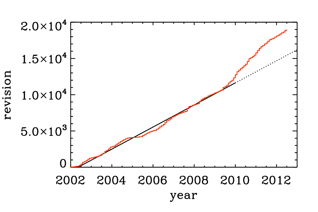
Fig. 3.5 Number of check-ins since 2002. Note again the linear increase with time, although in the last part of the time series there is a notable speed-up.

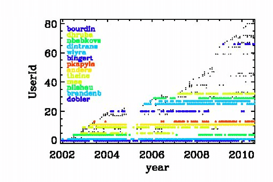
Fig. 3.6 Check-ins since 2002 per user. Users with more than 100 check-ins are color coded.

The Pencil Code check-ins occur regularly all the time. By the Pencil Code User Meeting 2010 we have arrived at a revision number of 15,000. In February 2017, the number of check-ins has risen to 26,804; see https://github.com/pencil-code/pencil-code. Major code changes are nowadays being discussed by the Pencil Code Steering Committee (PCSC website). The increase of the revision number with time is depicted in Fig. 3.5. The number of Pencil Code developers increases too (Fig. 3.6), but the really active ones are getting rare. This may indicate that new users can produce new science with the code as it is, but it may also indicate that it is getting harder to understand the code. How to understand the code will be discussed in the next section.

3.1. Understanding the code

Understanding the code means looking through the code. This is not normally done by just printing out the entire code, but by searching your way through the code in order to address your questions. The general concept will be illustrated here with an example.

3.1.1. Example: how is the continuity equation being solved?

All the physics modules are solved in the routine pde, which is located in the file and module Equ. Somewhere in the pde subroutine you find the line

call dlnrho_dt(f,df,p)

This means that here the part belonging to \(\partial\ln\rho/\partial t\) is being assembled. Using the grep command you will find that this routine is located in the module density, so look in there and try to understand the pieces in this routine. We quickly arrive at the following crucial part of code,

!
!  Continuity equation.
!
      if (lcontinuity_gas) then
        if (ldensity_nolog) then
          df(l1:l2,m,n,irho)   = df(l1:l2,m,n,irho)   - p%ugrho - p%rho*p%divu
        else
          df(l1:l2,m,n,ilnrho) = df(l1:l2,m,n,ilnrho) - p%uglnrho - p%divu
        endif
      endif

where, depending on some logicals that tell you whether the continuity equation should indeed be solved and whether we do want to solve for the logarithmic density and not the actual density, the correct right hand side is being assembled. Note that all these routines always only add to the existing df(l1:l2,m,n,ilnrho) array and never reset it. Resetting df is only done by the timestepping routine. Next, the pieces p%uglnrho and p%divu are being subtracted. These are pencils that are organized in the structure with the name p. The meaning of their names is obvious: uglnrho refers to \(\uv\cdot\nabla\ln\rho\) and divu refers to \(\nabla\cdot\uv\). In the subroutine pencil_criteria_density you find under which conditions these pencils are requested. Using grep, you also find where they are calculated. For example p%uglnrho is calculated in density.f90; see

call u_dot_grad(f,ilnrho,p%glnrho,p%uu,p%uglnrho,UPWIND=lupw_lnrho)

So this is a call to a subroutine that calculates the \(\uv\cdot\nabla\) operator, where there is the possibility of Upwinding, but this is not the default. The piece divu is calculated in hydro.f90 in the line

!
!  Calculate uij and divu, if requested.
!
      if (lpencil(i_uij)) call gij(f,iuu,p%uij,1)
      if (lpencil(i_divu)) call div_mn(p%uij,p%divu,p%uu)

Note that the divergence calculation uses the velocity gradient matrix as input, so no new derivatives are recalculated. Again, using grep, you will find that this calculation and many other ones happen in the module and file sub.f90. The various derivatives that enter here have been calculated using the gij routine, which calls the der routine, e.g., like so

k1=k-1
do i=1,3
  do j=1,3
    if (nder==1) then
      call der(f,k1+i,tmp,j)

For all further details you just have to follow the trail. So if you want to know how the derivatives are calculated, you have to look in deriv.f90, and only here is it where the indices of the f array are being addressed.

If you are interested in magnetic fields, you have to look in the file magnetic.f90. The right hand side of the equation is assembled in the routine

!***********************************************************************
    subroutine daa_dt(f,df,p)
!
!  Magnetic field evolution.
!
!  Calculate dA/dt=uxB+3/2 Omega_0 A_y x_dir -eta mu_0 J.
!  For mean field calculations one can also add dA/dt=...+alpha*bb+delta*WXJ.
!  Add jxb/rho to momentum equation.
!  Add eta mu_0 j2/rho to entropy equation.
!

where the header tells you already a little bit of what comes below. It is also here where ohmic heating effects and other possible effects on other equations are included, e.g.,

!
!  Add Ohmic heat to entropy or temperature equation.
!
      if (lentropy .and. lohmic_heat) then
        df(l1:l2,m,n,iss) = df(l1:l2,m,n,iss) &
                          + etatotal*mu0*p%j2*p%rho1*p%TT1
      endif

We leave it at this and encourage the user to do similar inspection work on a number of other examples. If you think you find an error, file a ticket at http://code.google.com/p/pencil-code/issues/list. You can of course also repair it!

3.2. Adapting the code

3.2.1. The PENCIL CODE coding standard

As with any code longer than a few lines the appearance and layout of the source code is of the utmost importance. Well laid out code is more easy to read and understand and as such is less prone to errors.

A consistent coding style has evolved in the PENCIL CODE and we ask that those contributing try to be consistent for everybody’s benefit. In particular, it would be appreciated if those committing changes of existing code via svn follow the given coding style.

There are not terribly many rules and using existing code as a template is usually the easiest way to proceed. In short the most important rules are:

• tab characters do not occur anywhere in the code (in fact the use of tab character is an extension to the Fortran standard).

• Code in any delimited block, e.g., if statements, do loops, subroutines etc., is indented be precisely 2 spaces. E.g.

  if (lcylindrical) then
    call fatal_error('del2fjv','del2fjv not implemented')
  endif
  

• continuation lines (i.e. the continuation part of a logical line that is split using the & sign) are indented by 4 spaces. E.g. (note the difference from the previous example)

  if (lcylindrical) &
      call fatal_error('del2fjv','del2fjv not implemented')
  [...]
  

• There is always one space separation between ‘if’ and the criterion following in parenthesis:

  if (ldensity_nolog) then
    rho=f(l1:l2,m,n,irho)
  endif
  

  This is wrong:

  if(ldensity_nolog) then   ! WRONG
    rho=f(l1:l2,m,n,irho)
  endif
  

• In general, try to follow common practice used elsewhere in the code. For example, in the code fragment above there are no empty spaces within the mathematical expressions programmed in the code. A unique convention helps in finding certain expressions and patterns in the code. However, empty spaces are often used after commas and semicolons, for examples in name lists.

• Relational operators are written with symbols (==, /=, <, <=, >, >=), not with characters (.eq., .ne., .lt., .le., .gt., .ge.).

• In general all comments are placed on their own lines with the ! appearing in the first column. It can be omitted in empty lines, but is yet recommended to be set in empty lines surrounding comments.

• All subroutine/functions begin with a standard comment block describing what they do, when and by whom they were created and when and by whom any non-trivial modifications were made.

• Lines longer that ~100 characters should be explicitly wrapped using the & character, unless there is a block of longer lines that can only be read easily when they are not wrapped. Always add one whitespace before the & character.

These and other issues are discussed in more depth and with examples in Appendix Appendix B: Coding standard, and in particular in Sect. manApBCodingStandard.

3.2.2. Adding new output diagnostics

With the implementation of new physics and the development of new procedures it will become necessary to monitor new diagnostic quantities that have not yet been implemented in the code. In the following, we describe the steps necessary to set up a new diagnostic variable.

This is nontrivial as, in order to keep latency effects low on multi-processor machines, the code minimizes the number of global reduction operations by assembling all quantities that need the maximum taken in fmax, and those that need to be summed up over all processors (mostly for calculating mean quantities) in fsum (see subroutine diagnostic in file src/equ.f90).

As a sample variable, let us consider jbm (the volume average <j · B>). Only the module magnetic will be affected, as you can see (the diagnostic quantity jbm is already implemented) with:

unix> grep -i jbm src/*.f90

If we pretend for the sake of the exercise that no trace of jbm was in the code, and we were only now adding it, we would need to do the following:

1. add the variable idiag_jbm to the module variables of Magnetic in both magnetic.f90 and nomagnetic.f90:

   integer :: idiag_jbm=0
   

   The variable idiag_jbm is needed for matching the position of jbm with the list of diagnostic variables specified in print.in.

2. in the subroutine daa_dt in magnetic.f90, declare and calculate the quantity jb (the average of which will be jbm), and call sum_mn_name:

   real, dimension (nx) :: jb  ! jj·BB
   [...]
   if (ldiagnos) then          ! only calculate if diagnostics is required
     if (idiag_jbm/=0) then    ! anybody asked for jbm?
       call dot_mn(jj,bb,jb)   ! assuming jj and bb are known
       call sum_mn_name(jb,i_jbm)
     endif
   endif
   

3. in the subroutine rprint_magnetic in both magnetic.f90, add the following:

   !
   !  reset everything in case of RELOAD
   !  (this needs to be consistent with what is defined above!)
   !
   if (lreset) then  ! need to reset list of diagnostic variables?
     [...]
     idiag_jbm=0
     [...]
   endif
   !
   !  check for those quantities that we want to evaluate online
   !
   do iname=1,nname
     [...]
     call parse_name(iname,cname(iname),cform(iname),'jbm',idiag_jbm)
     [...]
   enddo
   [...]
   !
   !  write column, i_XYZ, where our variable XYZ is stored
   !
   [...]
   write(3,*) 'i_jbm=',idiag_jbm
   [...]
   

4. in the subroutine rprint_magnetic in nomagnetic.f90, add the following (newer versions of the code may not require this any more):

   !
   !  write column, i_jbm, where our variable jbm is stored
   !  idl needs this even if everything is zero
   !
   [...]
   write(3,*) 'i_jbm=',idiag_jbm
   [...]
   

5. and don’t forget to add your new variable to print.in:

   jbm(f10.5)
   

If, instead of a mean value, you want a new maximum quantity, you need to replace sum_mn_name() by max_mn_name().

Sect. One-dimensional output averaged in two dimensions describes how to output horizontal averages of the magnetic and velocity fields. New such averages can be added to the code by using the existing averaging procedures calc_bmz() or calc_jmz() as examples.

3.2.3. Output at one point in space

Various variables at one point can be printed on the command line. This is often important when you want to check for oscillations where the sign changes. You would not see it in the rms or max values. The extensions pt and p2 refer to variables that are taken from two particular points in space.

Note: this would need to be reworked if one later makes the output positions processor-dependent. At the moment, those positions are in that part of the mesh that is on the root processor.

The file pt_positions.dat lists the coordinate positions where the data is taken from.

3.2.4. The f-array

The f array is the largest array in the Pencil Code and its primary role is to store the current state of the timestepped PDE variables. The f-array and its slightly smaller counter part (the df-array; see below) are the only full size 3D arrays in the code. The f-array is of type real but PDEs for a complex variable may be solved by using two slots in the f-array. The actual size of the f-array is \(\rm{mx}\times\rm{my}\times\rm{mz}\times\rm{mfarray}\). Here, \(\rm{mfarray}=\rm{mvar}+\rm{maux}+\rm{mglobal}+\rm{mscratch}\) where \(\rm{mvar}\) refers to the number of real PDE variables.

As an example, we describe here how to put the time-integrated velocity, uut, into the f-array (see hydro.f90). If this is to be invoked, there must be the following call somewhere in the code:

call farray_register_auxiliary('uut',iuut,vector=3)

Here, iuut is the index of the variable uut in the f-array. Of course, this requires that maux is increased by 3, but in order to do this for a particular run only one must write a corresponding entry in the cparam.local file,

!                       -*-f90-*-    (for Emacs)
!  cparam.local
!
!** AUTOMATIC CPARAM.INC GENERATION ****************************************
! Declare (for generation of cparam.inc) the number of f array
! variables and auxiliary variables added by this module
!
! MAUX CONTRIBUTION 3
!
!***************************************************************************
!  Local settings concerning grid size and number of CPUs.
!  This file is included by cparam.f90
!
integer, parameter :: ncpus=1,nprocy=1,nprocz=ncpus/nprocy,nprocx=1
integer, parameter :: nxgrid=16,nygrid=nxgrid,nzgrid=nxgrid

This way such a change does not affect the memory usage for other applications where this addition to cparam.local is not made. In order to output this part of the f-array, one must write lwrite_aux=T in the init_pars of start.in. (Technically, lwrite_aux=T can also be invoked in run_pars of run.in, but this does not work at the moment.)

3.2.5. The df-array

The ‘df’ array is the second largest chunk of data in the Pencil Code. By using a 2N storage scheme (see S-2N-scheme) after Williamson [2Nstorage] the code only needs one more storage area for each timestepped variable on top of the current state stored in the f-array. As such, and in contrast to the f-array, the df-array is of size \(\rm{mx}\times\rm{my}\times\rm{mz}\times\rm{mvar}\). Like the df-array it is of type real. In fact the ghost zones of df are not required or calculated but having f- and df-arrays of the same size make the coding more transparent. For \(\rm{mx}\), \(\rm{my}\) and \(\rm{mz}\) large the wasted storage becomes negligible.

3.2.6. The fp-array

Similar to the ‘f’ array the code also has a ‘fp’ array which contains current states of all the particles. Like the f-array the fp-array also has a time derivative part, the dfp-array. The dimension of the fp-array is \(mpar_local\times mpvar\) where \(mpar_local\) is the number of particles in the local processor (for serial runs this is the total number of particles) and \(mpvar\) depends on the problem at hand. For example if we are solving for only tracer particles then \(mpvar=3\), for dust particles \(mpvar=6\). The sequence in which the slots in the fp-array are filled up depends on the sequence in which different particle modules are called from the particles_main.f90. The following are the relevant lines from particles_main.f90.

!***********************************************************************
    subroutine particles_register_modules()
!
!  Register particle modules.
!
!  07-jan-05/anders: coded
!
      call register_particles              ()
      call register_particles_radius       ()
      call register_particles_spin         ()
      call register_particles_number       ()
      call register_particles_mass         ()
      call register_particles_selfgrav     ()
      call register_particles_nbody        ()
      call register_particles_viscosity    ()
      call register_pars_diagnos_state     ()
!
    endsubroutine particles_register_modules
!***********************************************************************

The subroutine register_particles can mean either the tracer particles or dust particles. For the former the first three slots of the fp-array are the three spatial coordinates. For the latter the first six slots of the fp-array are the three spatial coordinates followed by the three velocity components. The seventh slot (or the fourth if we are using tracer particles) is the radius of the particle which can also change as a function of time as particles collide and fuse together to form bigger particles.

3.2.7. The pencil case

Variables that are derived from the basic physical variables of the code are stored in one-dimensional pencils of length nx. All the pencils that are defined for a given set of physics modules are in turn bundled up in a Fortran structure called p (or, more illustrative, the pencil case). Access to individual pencils happens through the variable p%name, where name is the name of a pencil, e.g., rho that is a derived variable of the logarithmic density lnrho.

The pencils provided by a given physics module are declared in the header of the file, e.g., in the Density module:

! PENCILS PROVIDED lnrho; rho; rho1; glnrho(3); grho(3); uglnrho; ugrho

Notice that the pencil names are separated with a semi-colon and that vector pencils are declared with “(3)” after the name, and “(3,3)” for a \(3\times3\) matrix. Before compiling the code, the script mkcparam collects the names of all pencils that are provided by the chosen physics modules. It then defines the structure p with slots for every single one of these pencils. The definition of the pencil case p is written in the include file cparam_pencils.inc. When the code is run, the actual pencils that are needed for the run are chosen based on the input parameters. This is done in the subroutines pencil_criteria_modulename that are present in each physics module. They are all called once before entering the time loop. In the pencil_criteria subroutines the logical arrays lpenc_requested, lpenc_diagnos, lpenc_diagnos2d, and lpenc_video are set according to the pencils that are needed for the given run. Some pencils depend on each other, e.g., uglnrho depends on uu and glnrho. Such interdependencies are sorted out in the subroutines pencil_interdep_modulename that are called after pencil_criteria_modulename.

In each time-step the values of the pencil logicals lpenc_requested, lpenc_diagnos, lpenc_diagnos2d, and lpenc_video are combined to one single pencil array lpencil which is different from time-step to time-step depending on, e.g., whether diagnostics or video output are done in that time-step. The pencils are then calculated in the subroutines calc_pencils_modulename. This is done before calculating the time evolution of the physical variables, as this depends very often on derived variables in pencils.

The centralized pencil calculation scheme is a guarantee that

• All pencils are only calculated once, and only once.

• Pencils are always calculated by the proper physics module.

Since the Pencil Code is a multipurpose code that has many different physics modules, it can lead to big problems if a module tries to calculate a derived variable that actually belongs to another module, because different input parameters can influence how the derived variables are calculated. One example is that the Density module can consider both logarithmic and non-logarithmic density, so if the Magnetic module calculates

rho = exp(f(l1:l2,m,n,ilnrho)

it is wrong if the Density module works with non-logarithmic density! The proper way for the Magnetic module to get to know the density is to request the pencil rho in pencil_criteria_magnetic.

3.2.7.1. Pencil check

To check that the correct pencils have been requested for a given run, one can run a pencil consistency check in the beginning of a run by setting the logical lpencil_check in &run_pars. The check is meant to see if

• All needed pencils have been requested

• All requested pencils are needed

The consistency check first calculates the value of df with all the requested pencils. Then the pencil requests are flipped one at a time – requested to not requested, not requested to requested. The following combination of events can occur:

• not requested → requested, df not changed The pencil is not requested and is not needed.

• not requested → requested, df changed The pencil is not requested, but is needed. The code stops.

• requested → not requested, df not changed The pencil is requested, but is not needed. The code gives a warning.

• requested → not requested, df changed The pencil is requested and is needed.

3.2.7.2. Adding new pencils

Adding a new pencil to the pencil case is trivial but requires a few steps.

• Declare the name of the pencil in the header of the proper physics module. Pencils names must appear come in a “;” separated list, with dimensions in parenthesis after the name [(3) for vector, (3,3) for matrix, etc.].

• Set interdependency of the new pencil (i.e. what other pencils does it depend on) in the subroutine pencil_interdep_modulename

• Make rule for calculating the pencil in calc_pencils_modulename

• Request the new pencil based on the input parameters in any relevant physics module

Remember that the centralized pencilation scheme is partially there to force the users of the code to think in general terms when implementing new physics. Any derived variable can be useful for a number of different physics problems, and it is important that a pencil is accessible in a transparent way to all modules.

3.2.8. Adding new physics: the Special module

If you want to add new physics to the code, you will in many cases want to add a new Special module. Doing so is relatively straightforward and there is even a special directory for such additions.

To create your own special module, copy nospecial.f90 from the src/ directory to a new name in the src/special/ directory. In many cases, users may want to put all new bits of physics, needed for the specific problem at hand, into a single special module. The name chosen for it should then relate to that problem. It is also possible to employ several (at present up to five) different special modules at a time in a single setup which allows to let naming follow the specific physics being implemented (for technicalities in this case, see the end of this section).

The first thing to do in your new module is to change the lspecial=.false. header to say lspecial=.true.

The file is heavily commented though all such comments can be removed as you go. You may implement any of the subroutines/function that exist in nospecial.f90 and those routines must have the names and parameters as in nospecial.f90. You do not however need to implement all routines, and you may either leave the dummy routines copied from nospecial.f90 or delete them all together (provided the “include ‘special_dummy.inc’” is kept intact at the end of the file). Beyond that, data and subroutines can be added to a special module as required, though only for use within that module.

There are routines in the special interface to allow you to add new equations, modify the existing equation, add diagnostics, add slices, and many more things. If you feel there is something missing extra hooks can easily be added — please contact the Pencil Code team for assistance.

You are encouraged to submit/commit your special modules to the Pencil Code source. When you have added new stuff to the code, don’t forget to mention this in the manual.tex file.

3.2.8.1. Using more than one special module at a time

Requires that the environment variables $MODULE_PREFIX, $MODULE_INFIX and $MODULE_SUFFIX are set properly at runtime. They can be derived from the qualified names of module functions which have in general the form:

\(\langle prefix \rangle \langle module name \rangle \langle infix \rangle \langle function name \rangle \langle suffix \rangle\)

with its details depending on the Fortran compiler used. These can be learned by employing the nm command, e.g.:

unix> nm src/general.o | more .

The environment variables are most conveniently set in the user’s .bashrc, .cshrc or a proper configuration file of the Pencil Code (section environment). In the Makefile.local file, the requested special modules are simply specified as a list of names:

SPECIAL = special/<module 1> special/<module 2> ...

In contrast to the case with only a single special module, where the namelists’ names are special_init_pars and special_run_pars, these are individualized for multiple special modules, viz. <module name>_init_pars etc. As explicit linking at runtime is employed for multiple special modules, code errors, which normally would break the build, show possibly up only at runtime and are hence hard to debug. Therefore in case of unclear runtime failure, it is useful to perform tests with only one of the special modules at a time, thus guaranteeing full linking at build time.

For example, when

SPECIAL  =   special/gravitational_waves_hTXk special/chiral_mhd

is used, the namelist that is usually referenced as

&special_run_pars
/

needs to be replaced by:

&gravitational_waves_hTXk_run_pars
/
&chiral_mhd_run_pars
/

Internally, a number of automatic replacements occur in the code. Code that is automatically modified in this way is also automatically unmodified while checking in changes to the repository. But to facilitate comparison with the original code, one can do the unmodification also oneself using the pencil-code/utils/axel/pc_mkspecial.sh command.

3.2.9. Adding switchable modules

In some cases where a piece of physics is thought to be more fundamental, useful in many situations or simply more flexibility is required it may be necessary to add a new module :name:`newphysics` together with the corresponding :name:`nonewphysics` module. The special modules follow the same structure as the rest of the switchable modules and so using a special module to prototype new ideas can make writing a new switchable module much easier.

For an example of a module involving a new variable (and PDE), the :name:`pscalar` module is a good prototype. The grep command

unix> grep -i pscalar src/*

gives you a good overview of which files you need to edit or add.

3.2.10. Adding your initial conditions: the InitialCondition module

Although the code has many initial conditions implemented, we now discourage such practice. We aim to eventually remove most of them. The recommended course of action is to make use of the InitialCondition module.

InitialCondition works pretty much like the Special module. To implement your own custom initial conditions, copy the file noinitial_condition.f90 from the src/ to src/initial_condition, with a new, descriptive name.

The first thing to do in your new module is to change the linitialcondition=.false. header to say linitialcondition=.true. Also, don’t forget to add ../ in front of the file names in include statements.

This file has hooks to implement a custom initial condition to most variables. After implementing your initial condition, add the line

INITIAL_CONDITION=initial_condition/myinitialcondition

to your src/Makefile.local file. Here, myinitialcondition is the name you gave to your initial condition file. Add also initial_condition_pars to the start.in file, just below init_pars. This is a namelist, which you can use to add whichever quantity your initial condition needs defined, or passed. You must also un-comment the relevant lines in the subroutines for reading and writing the namelists. For compiling reasons, these subroutines in noinitial_condition.f90 are dummies. The lines are easily identifiable in the code.

Check, e.g., the samples 2d-tests/baroclinic, 2d-tests/spherical_viscous_ring, or interlocked-fluxrings, for examples of how the module is used.

3.3. Testing the code

To maintain reproducibility despite sometimes quite rapid development, the Pencil Code is tested nightly on various architectures. The front end for testing are the scripts pc_auto-test and (possibly) pencil-test.

To see which samples would be tested, run

unix> pc_auto-test -l

to actually run the tests, use

unix> pc_auto-test

or

unix> pc_auto-test --clean

The latter compiles every test sample from scratch and currently (September 2009) takes about 2 hours on a mid-end Linux PC.

The pencil-test script is useful for cron jobs and allows the actual test to run on a remote computer. See How to set up periodic tests (auto-tests) below.

For a complete list of options, run pc_auto-test --help and/or pencil-test --help.

3.3.1. How to set up periodic tests (auto-tests)

To set up a nightly test of the Pencil Code, carry out the following steps.

1. Identify a host for running the actual tests (the work host) and one to initiate the tests and collect the results (the scheduling host). On the scheduling host, you should be able to:

   1. run cron jobs,

   2. ssh to the work host without password,

   3. publish HTML files (optional, but recommended),

   4. send e-mail (optional, but recommended).

   Work host and scheduling host can be the same (in this case, use pencil-test’s -l option), but often they will be two different computers.

2. [Recommended, but optional:] On the work host, check out a separate copy of the Pencil Code to reduce the risk that you start coding in the auto-test tree. In the following, we will assume that you checked out the code as ~/pencil-auto-test.

3. On the work host, make sure that the code finds the correct configuration file for the tests you want to carry out. [Elaborate on that: PENCIL_HOME/local_config and -f option; give explicit example]

   Remember that you can set up a custom host ID file for your auto-test tree under $PENCIL_HOME/config-local/hosts/.

4. On the scheduling host, use crontab -e to set up a :name:`cron` job similar to the following:

30 02 * * *  $HOME/pencil-auto-test/bin/pencil-test \
    -D $HOME/pencil-auto-test \
    --use-pc_auto-test \
    -N15 -Uc -rs \
    -T $HOME/public_html/pencil-code/tests/timings.txt \
    -t 15m
    -m <email1@inter.net,email2@inter.net,...> \
    <work-host.inter.net> \
    -H > $HOME/public_html/pencil-code/tests/nightly-tests.html

Note

This has to be one long line. The backslash characters are written only for formatting purposes for this manual (you cannot use them in a crontab file).

Note

You will have to adapt some parameters listed here and may want to modify a few more:

• -D <dir>: Sets the directory (on the work host) to run in.

• -T <file>: If this option is given, append a timing statistics line for each test to the given file.

• --use-pc: You want this option (and at some point, it will be the default).

• -t 15m: Limit the time for start.x and run.x to 15 minutes.

• -N 15: Run the tests at nice level 15 (may not have an effect for MPI tests).

• -Uc: Do svn update and pc_build --cleanall before compiling.

• work-host.inter.net|-l: Replace this with the remote host that is to run the tests. If you want to run locally, write -l instead.

• -H: Output HTML.

• > $HOME/public_html/pencil-code/tests/nightly-tests.html: Write output to the given file.

If you want to run fewer or more tests, you can use the -Wa,--max-level option:

-Wa,--max-level=3

will run all tests up to (and including) level 3. The default corresponds to -Wa,--max-level=2.

For a complete listing of pencil-test options, run

unix> pencil-test --help

3.3.2. Auto-tests with systemd

On modern Linux systems, you can use systemd (instead of cron) to run periodic auto-tests. You need to create a couple of files in ~/.config/systemd/user/:

pencil_test.service [1] :

[Unit]
Description=Pencil-code test

[Service]
Type=simple
Environment="PENCIL_HOME=%h/.software/pencil-code-for-tests"
ExecStart=%h/.software/pencil-code-for-tests/bin/pencil-test \
    -N 15 --update --html --clean --local --use-pc_auto-test \
    --auto-test-options="--max-level=3 --script-tests=python --time-limit=5m"
StandardOutput=truncate:%h/public_html/pencil_tests/master_full.html

(the backslashes can be left as-is) and pencil_test.timer:

[Unit]
Description=Run pencil test daily at 10pm

[Timer]
OnCalendar=*-*-* 22:00:00
Persistent=True

[Install]
WantedBy=timers.target

After creating these files, run

systemctl --user enable pencil_test.timer
systemctl --user start pencil_test.timer

[1]

Options and filepaths may need to be modified; note that %h is used to denote the user’s home directory.

3.3.3. Testing the postprocessing modules

Some of the samples contain additional scripts that test the Python and IDL postprocessing modules. They are not checked by pc_auto-test by default; to include these tests, use the --script-tests option, e.g.:

pc_auto-test --max-level=3 --script-tests=python

The Python postprocessing modules contain an additional set of quick tests that can be invoked as described in PENCIL_HOME/python/tests/README.md.

3.4. Useful internals

3.4.1. Global variables

The following variables are defined in cdata.f90 and are available in any routine that uses the module Cdata.

Variable	Meaning
Real
t	simulated time t.
integer
n[xyz]grid	global number of grid points (excluding ghost cells) in x, y and z direction.
nx, ny, nz	number of grid points (excluding ghost cells) as seen by the current processor, i.e., ny=nygrid/nprocy, etc.
mx, my, mz	number of grid points seen by the current processor, but including ghost cells. Thus, the total box for the ivar-th variable (on the given processor) is given by f(1:mx,1:my,1:mz,ivar).
l1, l2	smallest and largest x-index for the physical domain (i.e., excluding ghost cells) on the given processor.
m1, m2	smallest and largest y-index for physical domain.
n1, n2	smallest and largest z-index for physical domain, i.e., the physical part of the ivar-th variable is given by f(l1:l2,m1:m2,n1:n2,ivar)
m, n	pencil indexing variables: During each time-substep the box is traversed in x-pencils of length mx such that the current pencil of the ivar-th variable is f(l1:l2,m,n,ivar).
logical
lroot	true only for MPI root processor.
lfirst	true only during first time-substep of each time step.
headt	true only for very first full time step (comprising 3 substeps for the 3rd-order Runge–Kutta scheme) on root processor.
headtt	= (lfirst .and. lroot): true only during very first time-substep on root processor.
lfirstpoint	true only when the very first pencil for a given time-substep is processed, i.e., for the first set of (m,n), which is probably (3,3).
lout	true when diagnostic output is about to be written.

3.4.2. Subroutines and functions

output(file,a,nv)	(module Cdata): Write (in each procN/ directory) the content of the global array a to a file called file, where a has dimensions mx \(\times\) my \(\times\) mz \(\times\) nv or mx \(\times\) my \(\times\) mz if nv=1.
output_pencil(file,a,nv)	(module IO): Same as output(), but for a pencil variable, i.e. an auxiliary variable that only ever exists on a pencil (e.g., the magnetic field strength bb in magnetic.f90, or the squared sound speed cs2 in entropy.f90). The file has the same structure as those written by output(), because the values of a on the different pencils are accumulated in the file. This involves a quite nontrivial access pattern to the file and has thus been coded in C (src/debug_c.c).
cross(a,b,c)	(module Sub): Calculate the cross product of two vectors a and b and store in c. The vectors must either all be of size mx \(\times\) my \(\times\) mz \(\times\) 3 (global arrays), or of size nx×3 (pencil arrays).
dot(a,b,c)	(module Sub): Calculate the dot product of two vectors a and b and store in c. The vectors must either be of size mx \(\times\) my \(\times\) mz \(\times\) 3 (a and b) and mx \(\times\) my \(\times\) mz \(\times\) (c), or of size nx :math:`times`3 (a and b) and nx (c).
dot2(a,c)	(module Sub): Same as dot(a,a,c).

3.5. References

[Abramowitz-Stegun]

Abramowitz, A., & Stegun, I. A. (1984). Pocketbook of Mathematical Functions. Harri Deutsch, Frankfurt.

[BHB11]

Babkovskaia, N., Haugen, N. E. L., & Brandenburg, A. (2011). J. Comp. Phys., 230(1), 12. A high-order public domain code for direct numerical simulations of turbulent combustion. (arXiv:1005.5301)

[BB14]

Barekat, A., & Brandenburg, A. (2014). Astron. Astrophys., 571, A68. “Near-polytropic stellar simulations with a radiative surface.”

[Ref-2]

Brandenburg, A. (2001). Astrophys. J., 550, 824–840. “The inverse cascade and nonlinear alpha-effect in simulations of isotropic helical hydromagnetic turbulence.”

[Ref-1]

Brandenburg, A. (2003). In Advances in non-linear dynamos (A. Ferriz-Mas & M. Núñez Jiménez, Eds.), The Fluid Mechanics of Astrophysics and Geophysics, Vol. 9, pp. 269–344. Taylor & Francis, London and New York. Available at http://arXiv.org/abs/astro-ph/0109497

[Ref-4]

Brandenburg, A., & Dobler, W. (2001). Astron. Astrophys., 369, 329–338. “Large scale dynamos with helicity loss through boundaries.”

[BH01]

Brandenburg, A., & Hazlehurst, J. (2001). Astron. Astrophys., 370, 1092–1102. “Evolution of highly buoyant thermals in a stratified layer.”

[BK17]

Brandenburg, A., & Kahniashvili, T. (2017). Phys. Rev. Lett., 118, 055102. “Classes of hydrodynamic and magnetohydrodynamic turbulent decay.”

[BHKRS21]

Brandenburg, A., He, Y., Kahniashvili, T., Rheinhardt, M., & Schober, J. (2021). Astrophys. J., 911, 110. “Gravitational waves from the chiral magnetic effect.”

[BS02]

Brandenburg, A., & Sarson, G. R. (2002). Phys. Rev. Lett., 88, 055003. “The effect of hyperdiffusivity on turbulent dynamos with helicity.”

[BDS02]

Brandenburg, A., Dobler, W., & Subramanian, K. (2002). Astron. Nachr., 323, 99–122. “Magnetic helicity in stellar dynamos: new numerical experiments.”

[BEO96]

Brandenburg, A., Enqvist, K., & Olesen, P. (1996). Phys. Rev. D, 54, 1291–1300. “Large-scale magnetic fields from hydromagnetic turbulence in the very early universe.”

[BJNRST96]

Brandenburg, A., Jennings, R. L., Nordlund, Å., Rieutord, M., Stein, R. F., & Tuominen, I. (1996). J. Fluid Mech., 306, 325–352. “Magnetic structures in a dynamo simulation.”

[BKMRPTV17]

Brandenburg, A., Kahniashvili, T., Mandal, S., Roper Pol, A., Tevzadze, A. G., & Vachaspati, T. (2017). Phys. Rev. D, 96, 123528. “Evolution of hydromagnetic turbulence from the electroweak phase transition.”

[BMS95]

Brandenburg, A., Moss, D., & Shukurov, A. (1995). MNRAS, 276, 651–662. “Galactic fountains as magnetic pumps.”

[BNST95]

Brandenburg, A., Nordlund, Å., Stein, R. F., & Torkelsson, U. (1995). Astrophys. J., 446, 741–754. “Dynamo-generated turbulence and large scale magnetic fields in a Keplerian shear flow.”

[Collatz66]

Collatz, L. (1966). The numerical treatment of differential equations. Springer-Verlag, New York, p. 164.

[Dobler06]

Dobler, W., Stix, M., & Brandenburg, A. (2006). Astrophys. J., 638, 336–347. “Convection and magnetic field generation in fully convective spheres.”

[Dur08]

Durrer, R. (2008). The Cosmic Microwave Background. Cambridge University Press.

[Gammie2001]

Gammie, C. F. (2001). Astrophys. J., 553, 174–183. “Nonlinear outcome of gravitational instability in cooling, gaseous disks.”

[GNG87]

Goodman, J., Narayan, R., & Goldreich, P. (1987). Month. Not. Roy. Soc., 225, 695–711. “The stability of accretion tori — II. Nonlinear evolution to discrete planets.”

[HB04a]

Haugen, N. E. L., & Brandenburg, A. (2004). Phys. Rev. E, 70, 026405. “Inertial range scaling in numerical turbulence with hyperviscosity.”

[HockneyEastwood1981]

Hockney, R. W., & Eastwood, J. W. (1981). Computer Simulation Using Particles. McGraw-Hill, New York.

[HTM84]

Hurlburt, N. E., Toomre, J., & Massaguer, J. M. (1984). Astrophys. J., 282, 557–573. “Two-dimensional compressible convection extending over multiple scale heights.”

[kim87]

Kim, J., Moin, P., & Moser, R. (1987). J. Fluid Mech., 177, 133. “Turbulence statistics in fully developed channel flow at low Reynolds number.”

[KW90]

Kippenhahn, R., & Weigert, A. (1990). Stellar structure and evolution. Springer, Berlin.

[KR80]

Krause, F., & Rädler, K.-H. (1980). Mean-Field Magnetohydrodynamics and Dynamo Theory. Akademie-Verlag, Berlin; also Pergamon Press, Oxford.

[Lele92]

Lele, S. K. (1992). J. Comp. Phys., 103, 16–42. “Compact finite difference schemes with spectral-like resolution.”

[MTW]

Misner, C. W., Thorne, K. S., & Wheeler, J. A. (1973). Gravitation. San Francisco: W. H. Freeman and Co., p. 213.

[MTBM09]

Mitra, D., Tavakol, R., Brandenburg, A., & Moss, D. (2009). Astrophys. J., 697, 923–933. “Turbulent dynamos in spherical shell segments of varying geometrical extent.” (arXiv:0812.3106)

[NG95]

Nordlund, Å., & Galsgaard, K. (1995). A 3D MHD code for Parallel Computers. Available at http://www.astro.ku.dk/~aake/NumericalAstro/papers/kg/mhd.ps.gz

[NS90]

Nordlund, Å., & Stein, R. F. (1990). Comput. Phys. Commun., 59, 119. “3-D simulations of solar and stellar convection and magnetoconvection.”

[Ole97]

Olesen, P. (1997). Phys. Lett. B, 398, 321. “Inverse cascades and primordial magnetic fields.”

[NR]

Press, W., Teukolsky, S., Vetterling, W., & Flannery, B. (1996). Numerical Recipes in Fortran 90 (2nd ed.). Cambridge.

[SH88]

Stanescu, D., & Habashi, W. G. (1988). J. Comp. Phys., 143, 674. “2N-storage low dissipation and dispersion Runge–Kutta schemes for computational acoustics.”

[2Nstorage]

Williamson, J. H. (1980). J. Comp. Phys., 35, 48. “Low-storage Runge–Kutta schemes.”

[JOSS]

Pencil Code Collaboration. (2021). J. Open Source Software, 6, 2807. “The Pencil Code, a modular MPI code for partial differential equations and particles: multipurpose and multiuser-maintained.”

[Porter22]

Porter, T. A., Jóhannesson, G., & Moskalenko, I. V. (2022). Astrophys. J. Supp., 262, 30. “The GALPROP Cosmic-ray Propagation and Nonthermal Emissions Framework: Release v57.”

[mcmodel]

Intel. Fortran Compiler Developer Guide and Reference – mcmodel. https://software.intel.com/en-us/fortran-compiler-developer-guide-and-reference-mcmodel