2. Part 1: Using the PENCIL CODE

2.1. System requirements

To use the code, you will need the following:

1. Absolutely needed:

   • F95 compiler

   • C compiler

2. Used heavily (if you don’t have one of these, you will need to adjust many things manually):

   • a Unix/Linux-type system with make and csh

   • Perl (remember: if it doesn’t run Perl, it’s not a computer)

3. The following are dispensable, but enhance functionality in one way or the other:

   • an MPI implementation (for parallelization on multiprocessor systems)

   • DX alias OpenDX or data explorer (for 3-D visualization of results)

   • IDL (for visualization of results; the 7-minute demo license will do for many applications)

2.2. Obtaining the code

The code is now distributed via GitHub repository, where you can either download a tarball, or, preferably, download it via svn or git. In Iran and some other countries, GitHub is not currently available. To alleviate this problem, we have made a recent copy available on http://www.nordita.org/software/pencil-code/. If you want us to update this tarball, please contact us.

To ensure at least some level of stability of the svn/git versions, a set of test problems (listed in $PENCIL_HOME/bin/auto-test) are routinely tested. This includes all problems in $PENCIL_HOME/samples. See S-Testing for details.

2.2.1. Obtaining the code via git or svn

1. Many machines have svn installed (try svn -v or which svn). On Ubuntu, for example, svn comes under the package name subversion.

2. The code is now saved under GitHub; git can be obtained in Linux by typing:

   sudo apt-get install git
   

3. Unless you are a privileged user with write access, you can download the code with the command:

   git clone https://github.com/pencil-code/pencil-code.git
   

   or:

   svn checkout https://github.com/pencil-code/pencil-code/trunk/ \
   pencil-code --username MY_GITHUB_USERNAME
   

   In order to push your changes to the repository, you have to ask the maintainer of the Pencil Code for push access (to become a contributor), or submit a pull request to the maintainer of the code.

   Be sure to run auto-test before you check anything back in. It can be very annoying for someone else to figure out what’s wrong, especially if you are just testing something else. At the very least, you should do:

   pc_auto-test --level=0 --no-pencil-check -C
   

   This allows you to run just the 2 most essential tests, starting with no-modules and then most-modules.

See also Download the Pencil Code for general information on obtaining the code.

2.2.2. Updating via svn or git

Independent of how you installed the code in the first place (from tarball or via svn/git), you can update your version using svn/git. If you have done nontrivial alterations to your version of the code, you ought to be careful about upgrading: although svn/git is an excellent tool for distributed programming, conflicts are quite possible, since many developers may touch many parts of the code while developing it further. Thus, despite the fact that the code is under svn/git, you should probably back up your important changes before upgrading.

Here is the upgrading procedure for git:

1. Perform a git update of the tree:

   unix> git pull \
   

2. Fix any conflicts you encounter and make sure the examples in the directory samples/ are still working.

Here is the upgrading procedure for svn:

1. Perform a svn update of the tree:

   unix> pc_svnup \
   

2. Fix any conflicts you encounter and make sure the examples in the directory samples/ are still working.

If you have made useful changes, please contact one of the (currently) 10 “Contributors” (listed under GitHub) who can give you push or check-in permission. Be sure to have sufficient comments in the code and please follow our standard coding conventions explained in programming-style. There is also a script to check and fix the most common style breaks, pc_codingstyle.

2.2.3. Getting the last validated version

The script pc_svnup accepts arguments -val or -validated, which means that the current changes on a user’s machine will be merged into the last working version. This way every user can be sure that any problems with the code must be due to the current changes done by this user since the last check-in.

Examples:

$ pc_svnup -src -s -validated

brings all files in src/ under $PENCIL_HOME to the last validated status, and merges all your changes into this version. This allows you to work with this, but in order to check in your changes you have to update everything to the most recent status first, i.e.

$ pc_svnup -src

Your own changes will be merged into this latest version as before.

Note

The functionality of the head of the trunk should be preserved at all times. However, accidents do happen. For the benefit of all other developers, any errors should be corrected within 1-2 hours. This is the reason why the code comes with a file pencil-code/license/developers.txt, which should contain contact details of all developers. The pc_svnup -val option allows all other people to stay away from any trouble.

2.2.4. Getting older versions

You may find that the latest svn version of the code produces errors. If you have reasons to believe that this is due to changes introduced on 27 November 2008 (to give an example), you can check out the version prior to this by specifying a revision number with svn update -r #####. One reason why one cannot always reproduce exactly the same situation too far back in time is connected with the fact that processor architecture and the compiler were different, resulting, e.g., in different rounding errors.

2.3. Getting started

To get yourself started, you should run one or several examples which are provided in one of the samples/ subdirectories. Note that you will only be able to fully assess the numerical solutions if you visualize them with IDL, DX, or other tools (see visualization).

2.3.1. Setup

2.3.1.1. Environment settings

The functionality of helper scripts and IDL routines relies on a few environment variables being set correctly. The simplest way to achieve this is to go to the top directory of the code and source one of the two scripts sourceme.csh or sourceme.sh (depending on the type of shell you are using):

csh> cd pencil-code
csh> source ./sourceme.csh

for tcsh or csh users; or

sh> cd pencil-code
sh> . ./sourceme.sh

for users of bash, Bourne shell, or similar shells. You should get output similar to:

PENCIL_HOME = </home/dobler/f90/pencil-code>
Adding /home/dobler/f90/pencil-code/bin to PATH

Apart from the PATH variable, the environment variable IDL_PATH is set to something like ./idl:../idl:+$PENCIL_HOME/idl:./data:<IDL_DEFAULT>.

Note

The <IDL_DEFAULT> mechanism does not work for IDL versions 5.2 or older. In this case, you will have to edit the path manually, or adapt the sourceme scripts.

Note

If you don’t want to rely on the sourceme scripts’ (quite heuristic) ability to correctly identify the code’s main directory, you can set the environment variable PENCIL_HOME explicitly before you run the source command.

Note

Do not just source the sourceme script from your shell startup file (~/.cshrc or ~/.bashrc), because it outputs a few lines of diagnostics for each sub-shell, which will break many applications. To suppress all output, follow the instructions given in the header documentation of sourceme.csh and sourceme.sh. Likewise, output from other files invoked by source should also be suppressed.

Note

The second time you source sourceme, it will not add anything to your PATH variable. This is on purpose to avoid cluttering of your environment: you can source the file as often as you like (in your shell startup script, then manually and in addition in some script you have written), without thinking twice. If, however, at the first sourcing, the setting of PENCIL_HOME was wrong, this mechanism would keep you from ever adding the right directory to the PATH. In this case, you need to first undefine the environment variable PENCIL_HOME:

csh> unsetenv PENCIL_HOME
csh> source ./sourceme.csh
or
sh> unset PENCIL_HOME
sh> . ./sourceme.sh

Note

If you want to be able to easily handle multiple versions/branches of Pencil, you can use the modulefile mechanism that is used on most clusters to load libraries and programs. Create a file at, say, $HOME/.modulefiles/pencil-local with the following contents:

#%Module4.6#####################################################################

proc ModulesHelp {} {
  global version prefix

  puts stderr "\tmodules - loads the modules software"
  puts stderr "& application environment"
  puts stderr "\n\tThis adds $prefix/* to several of the"
  puts stderr "\tenvironment variables."
  puts stderr "\n\tVersion $version\n"
}

module-whatis   "Environment setup for the Pencil code"

#change the following line according to the location of your local copy of Pencil
setenv          PENCIL_HOME     $env(HOME)/.software/pencil-code

setenv          _sourceme_quiet 1
source-sh       bash            $env(PENCIL_HOME)/sourceme.sh
unsetenv        _sourceme_quiet

To your ~/.bashrc, add:

MODULEPATH=$HOME/.modulefiles:$MODULEPATH

If you now open a new shell and run module avail, you will find the pencil-local module created above listed as an option. This requires version 4.6 of the modules program.

2.3.1.2. Linking scripts and source files

With your environment set up correctly, you can now go to the directory you want to work in and set up subdirectories and links. This is accomplished by the script pc_setupsrc, which is located in $PENCIL_HOME/bin and is thus now in your executable path.

For concreteness, let us assume you want to use samples/conv-slab as your run directory, i.e., you want to run a three-layer slab model of solar convection. You then do the following:

unix> cd samples/conv-slab
unix> pc_setupsrc
src already exists
2 files already exist in src

The script has linked a number of scripts from $PENCIL_HOME/bin, generated a directory src for the source code and linked the Fortran source files (plus a few more files) from $PENCIL_HOME/src to that directory:

unix> ls -F
reference.out  src/
start.csh@     run.csh@  getconf.csh@
start.in       run.in    print.in

2.3.1.3. Adapting Makefile.src

This step requires some input from you, but you only have to do this once for each machine you want to run the code on. See Adapting Makefile.src [obsolete; see Sect.:ref:man1_configuration] for a description of the steps you need to take here.

Note

If you are lucky and use compilers similar to the ones we have, you may be able to skip this step; but blame yourself if things don’t compile, then. If not, you can run make with explicit flags, see S-make-flags and in particular Table Compiler flags for common compilers.

2.3.1.4. Running make

Next, you run make in the src subdirectory of your run directory. Since you are using one of the predefined test problems, the settings in src/Makefile.local and src/cparam.local are all reasonable, and you just do:

unix> make

If you have set up the compiler flags correctly, compilation should complete successfully.

2.3.1.5. Choosing a data directory

The code will by default write data like snapshot files to the subdirectory data of the run directory. Since this will involve a large volume of IO operations (at least for large grid sizes), one will normally try to avoid writing the data via NFS.

The recommended way to set up a data directory is to generate a corresponding directory on the local disk of the computer you are running on and (soft-)link it to ./data. Even if the link is part of an NFS directory, all the IO operations will be local.

For example, if you have a local disk /scratch, you can do the following:

unix> mkdir -p /scratch/$USER/pencil-data/samples/conv-slab
unix> ln -s /scratch/$USER/pencil-data/samples/conv-slab ./data

This is done automatically by the pc_mkdatadir command which, in turn, is invoked when making a new run directory with the pc_newrun command, for example.

Even if you don’t have an NFS-mounted directory (say, on your notebook computer), it is probably still a good idea to have code and data well separated by a scheme like the one described above.

An alternative to symbolic links is to provide a file called datadir.in in the root of the run directory. This file should contain one line of text specifying the absolute or relative data directory path to use. This facility is useful if one wishes to switch one run directory between different data directories. It is suggested that in such cases symbolic links are again made in the run directory; then the datadir.in need contain only a short relative path.

2.3.1.6. Running the code

You are now ready to start the code:

unix> start.csh
Linux cincinnatus 2.4.18-4GB #1 Wed Mar 27 13:57:05 UTC 2002 i686 unknown
Non-MPI version
datadir = data
Fri Aug  8 21:36:43 CEST 2003
   src/start.x
CVS: io_dist.f90        v. 1.61         (brandenb  ) 2003/08/03 09:26:55
[...]
CVS: start.in           v. 1.4          (dobler    ) 2002/10/02 20:11:14
 nxgrid,nygrid,nzgrid=          32          32          32
 thermodynamics: assume cp=1

 uu: up-down
 piecewise polytropic vertical stratification (lnrho)
 init_lnrho: cs2bot,cs2top=   1.450000      0.3333330
 e.g., for ionization runs: cs2bot,cs2top not yet set
 piecewise polytropic vertical stratification (ss)

 start.x has completed successfully

 0.070u 0.020s 0:00.14 64.2%     0+0k 0+0io 180pf+0w

 Fri Aug  8 21:36:43 CEST 2003

This runs src/start.x to construct an initial condition based on the parameters set in start.in. This initial condition is stored in data/proc0/var.dat (and :data/proc1/var.dat, etc., if you run the multiprocessor version). It is fair to say that this is now a rather primitive routine; see pencil-code/idl/read for various reading routines. You can then visualize the data using standard IDL language.

If you visualize the profiles using IDL (see below), the result should bear some resemblance to Fig-pvert1, but with different values in the ghost zones (the correct values are set at run-time only) and a simpler velocity profile.

Now we run the code:

unix> run.csh

This executes src/run.x and carries out nt time steps, where nt and other run-time parameters are specified in run.in. On a decent PC (1.7 GHz), 50 time steps take about 10 seconds.

The relevant part of the code’s output looks like:

--it----t-------dt-------urms----umax----rhom------ssm-----dtc----dtu---dtnu---dtchi-
   0   0.34  6.792E-03  0.0060  0.0452  14.4708  -0.4478  0.978  0.013  0.207  0.346
  10   0.41  6.787E-03  0.0062  0.0440  14.4707  -0.4480  0.978  0.013  0.207  0.345
  20   0.48  6.781E-03  0.0064  0.0429  14.4705  -0.4481  0.977  0.012  0.207  0.345
  30   0.54  6.777E-03  0.0067  0.0408  14.4703  -0.4482  0.977  0.012  0.207  0.345
  40   0.61  6.776E-03  0.0069  0.0381  14.4702  -0.4482  0.977  0.011  0.207  0.346

The columns list:

• it: the number of the current time step

• t: the time

• dt: the time step

• urms: the rms velocity, urms = sqrt(<u^2>)

• umax: the maximum velocity, umax = max |u|

• rhom: the mean density, rhom = <rho>

• ssm: the mean entropy, ssm = <s>/cp

• dtc: the time step in units of the acoustic Courant step, dtc = dt * cs0 / dx_min

• dtu: the time step in units of the advective time step, dtu = dt / (c_delta_t * dx / max|u|)

• dtnu: the time step in units of the viscous time step, dtnu = dt / (c_delta_t_v * dx^2 / nu_max)

• dtchi: the time step in units of the conductive time step, dtchi = dt / (c_delta_t_v * dx^2 / chi_max)

The entries in this list can be added, removed or reformatted in the file print.in (see Sects. Diagnostic output and S-print.in-params). The output is also saved in data/time_series.dat and should be identical to the content of reference.out.

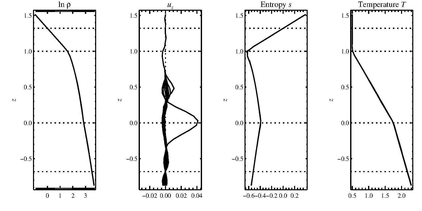
Fig. 2.1 Stratification of the three-layer convection model in samples/conv-slab after 50 timesteps (t=0.428). Shown are (from left to right) density rho, vertical velocity u_z, entropy s/cp and temperature T as functions of the vertical coordinate z for about ten different vertical lines in the computational box. The dashed lines denote domain boundaries: z < -0.68 is the lower ghost zone (points have no physical significance); -0.68 < z < 0 is a stably stratified layer (ds/dz > 0); 0 < z < 1 is the unstable layer (ds/dz < 0); 1 < z < 1.32 is the isothermal top layer; z > 1.32 is the upper ghost zone (points have no physical significance).

If you have IDL, you can visualize the stratification with (see Sect. IDL for details):

unix > idl
IDL >  pc_read_var,obj=var,/trimall
IDL >  tvscl,var,uu(*,*,0,0)

which shows u_x in the xy plane through the first meshpoint in the z direction.

The same can be achieved using Python (see Sect. Python Runtime Services for details) with:

unix > ipython3  # (or 'ipython', or just 'python')
python > import pencil as pc
python > from matplotlib import pylab as plt
python > var = pc.read.var(trimall=True)
python > plt.imshow(var.uu[0, 0, :, : ].T, origin='lower')

Note

If you want to run the code with MPI, you will probably need to adapt getconf.csh, which defines the commands and flags used to run MPI jobs (and which is sourced by the scripts start.csh and run.csh).

Try:

csh -v getconf.csh
or
csh -x getconf.csh

to see how getconf.csh makes its decisions. You would add a section for the host name of your machine with the particular settings. Since getconf.csh is linked from the central directory pencil-code/bin, your changes will be useful for all your other runs too.

2.3.2. Further tests

There are a number of other tests in the samples/ directory. You can use the script bin/auto-test to automatically run these tests and have the output compared to reference results.

2.4. Code structure

2.4.1. Directory tree

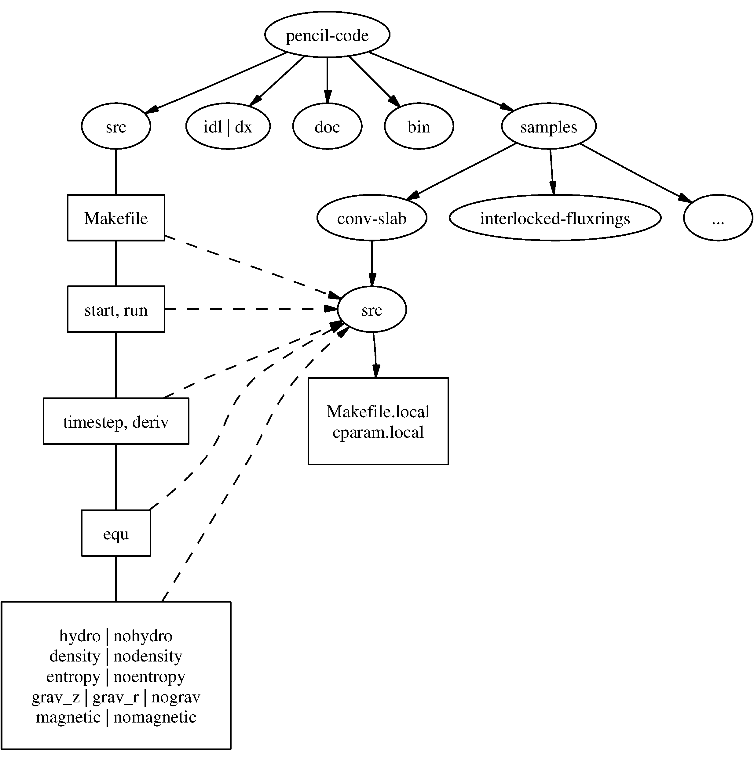
Fig. 2.2 The basic structure of the code

The overall directory structure of the code is shown in Fig. 2.2. Under pencil-code/, there are currently the following files and directories:

bin/   config/  doc/  idl/  license/  perl/   samples/      sourceme.sh  utils/
bugs/  dx/   lib/  misc/     README  sourceme.csh  src/         www/

Almost all of the source code is contained in the directory src/, but in order to encapsulate individual applications, the code is compiled separately for each run in a local directory src/ below the individual run directory, like e.,g.~:file:samples/conv-slab/src/.

It may be a good idea to keep your own runs also under SVN or CVS (which is older than but similar to SVN), but this would normally be a different repository. On the machine where you are running the code, you may want to check them out into a subdirectory of pencil-code/. For example, we have our own runs in a repository called pencil-runs, so we do:

unix> cd $PENCIL_HOME
unix> svn co runs pencil-runs

In this case, runs/ contains individual run directories, grouped in classes (like spher/ for spherical calculations, or kinematic/ for kinematic dynamo simulations). The current list of classes in our own pencil-runs/ repository is

1d-tests/   disc/          kinematic/  rings/
2d-tests/   discont/       Misc/       slab_conv/
3d-tests/   discussion/    OLD/        test/
buoy_tube/  forced/        pass_only/
convstar/   interstellar/  radiation/

The directory forced/ contains some forced turbulence runs (both magnetic and nonmagnetic); gravz/ contains runs with vertical gravity; rings/ contains decaying MHD problems (interlocked flux rings as initial condition, for example); and kinematic/ contains kinematic dynamo problems where the hydrodynamics is turned off entirely. The file samples/README should contain an up-to-date list and short description of the individual classes.footnote{Our pencil-runs/ directory also contains runs that were done some time ago. Occasionally, we try to update these, especially if we have changed names or other input conventions.}

The subdirectory src/ of each run directory contains a few local configuration files (currently these are Makefile.local and cparam.local) and possibly ctimeavg.local. To compile the samples, links the files *.f90, *.c and Makefile.src need to be linked from the top src/ directory to the local directory ./src. These links are set up by the script pc_setupsrc when used in the root of a run directory.

General-purpose visualization routines for IDL or DX are in the directories idl/ and dx/, respectively. There are additional and more specialized IDL directories in the different branches under pencil-runs/.

The directory doc/ contains this manual; bin/ contains a number of utility scripts (mostly written in C-shell and Perl), and in particular the start.csh, run.csh, and getconf.csh scripts. The .svn/ directory is used (you guessed it) by SVN, and is not normally directly accessed by the user; bugs/, finally, is used by us for internal purposes.

The files sourceme.csh and sourceme.sh will set up some environment variables — in particular PATH — and aliases/shell functions for your convenience. If you do not want to source one of these files, you need to make sure your IDL path is set appropriately (provided you want to use IDL) and you will need to address the scripts from bin/ with their explicit path name, or adjust your PATH manually.

2.4.2. Basic concepts

2.4.2.1. Data access in pencils

Unlike the CRAY computers that dominated supercomputing in the 80s and early 90s, all modern computers have a cache that constitutes a significant bottleneck for many codes. This is the case if large three-dimensional arrays are constantly used within each time step, which has the obvious advantage of working on long arrays and allows vectorization of elementary machine operations. This approach also implies conceptual simplicity of the code and allows extensive use of the intuitive F90 array syntax. However, a more cache-efficient way of coding is to calculate an entire time step (or substep of a multi-stage time-stepping scheme) only along a one-dimensional pencil of data within the numerical grid. This technique is more efficient for modern RISC processors: on Linux PCs and SGI workstations, for example, we have found a speed-up by about 60% in some cases. An additional advantage is a drastic reduction in temporary storage for auxiliary variables within each time step.

2.4.2.2. Modularity

Each run directory has a file src/Makefile.local in which you choose certain modules [1], which tell the code whether or not entropy, magnetic fields, hydrodynamics, forcing, etc.should be invoked. For example, the settings for forced turbulent MHD simulations are

HYDRO     =   hydro
DENSITY   =   density
ENTROPY   = noentropy
MAGNETIC  =   magnetic
GRAVITY   = nogravity
FORCING   =   forcing
MPICOMM   = nompicomm
GLOBAL    = noglobal
IO        =   io_dist
FOURIER   = nofourier

This file will be processed by make and the settings are thus assignments of make variables. Apart from the physics modules (equation of motion: yes, density [pressure]: yes, entropy equation: no, magnetic fields: yes, gravity: no, forcing: yes), a few technical modules can also be used or deactivated; in the example above, these are MPI (switched off), additional global variables (none), input/output (distributed), and FFT (not used). The table in Sect.~:ref:Tab-modules in the Appendix lists all currently available modules.

Note that most of these make variables must be set, but they will normally obtain reasonable default values in Makefile (so you only need to set the non-standard ones in Makefile.local). It is by using this switching mechanism through make that we achieve high flexibility without resorting to excessive amounts of cryptic preprocessor directives or other switches within the code.

Many possible combinations of modules have already been tested and examples are part of the distribution, but you may be interested in a combination which was never tried before and which may not work yet, since the modules are not fully orthogonal. In such cases, we depend on user feedback for fixing problems and documenting the changes for others.

[1]

We stress once more that we are not talking about F90 modules here, although there is some connection, as most of our modules define F90 modules: For example each of the modules gravity_simple, grav_r and nogravity defines a Fortran module Gravity.

2.4.3. Files in the run directories

2.4.3.1. start.in, run.in, print.in

These files specify the startup and runtime parameters (see Sects. Start and run parameters and S-all-run-params), and the list of diagnostic variables to print (see Diagnostic output). They specify the setup of a given simulation and are kept under svn svn in the individual samples/ directories.

You may want to check for the correctness of these configuration files by issuing the command pc_configtest.

2.4.3.2. datadir.in

If this file exists, it must contain the name of an existing directory, which will be used as data directory, i.e., the directory where all results are written. If datadir.in does not exist, the data directory is data/.

2.4.3.3. sn_series.in`

Formatted file containing the times and locations at which future supernova events will occur, using same format as sn_series.dat when lSN_list. (Only needed by the interstellar module.)

2.4.3.4. reference.out

If present, reference.out contains the output you should obtain in the given run directory, provided you have not changed any parameters. To see whether the results of your run are OK, compare time_series.dat to reference.out:

unix> diff data/time_series.dat reference.out

2.4.3.5. start.csh, run.csh, getconf.csh` [obsolete; see Sect. Configuring the code to compile and run on your computer]

These are links to $PENCIL_HOME/bin. You will be constantly using the scripts start.csh and run.csh to initialize the code. Things that are needed by both (like the name of the mpirun executable, MPI options, or the number of processors) are located in getconf.csh, which is never directly invoked.

2.4.3.6. src/

The src/ directory contains two local files, src/Makefile.local and src/cparam.local, which allow the user to choose individual modules (see Modularity) and to set parameters like the grid size and the number of processors for each direction. These two files are part of the setup of a given simulation and are kept under svn in the individual samples/ directories.

The file src/cparam.inc is automatically generated by the script mkcparam and contains the number of fundamental variables for a given setup.

All other files in src/ are either links to source files (and Makefile.src) in the $PENCIL_HOME/src directory, or object and module files generated by the compiler.

2.4.3.7. data/

This directory (the name of which will actually be overwritten by the first line of datadir.in, if that file is present; see datadir-in) contains the output from the code:

2.4.3.7.1. data/dim.dat

The global array dimensions.

2.4.3.7.2. data/legend.dat

The header line specifying the names of the diagnostic variables in time_series.dat.

2.4.3.7.3. data/time_series.dat

Time series of diagnostic variables (also printed to stdout). You can use this file directly for plotting with Gnuplot, IDL, Xmgrace or similar tools (see also S-Visualization).

2.4.3.7.4. data/tsnap.dat, data/tvid.dat

Time when the next snapshot VAR$N$ or animation slice should be taken.

2.4.3.7.5. data/params.log

Keeps a log of all your parameters: start.x writes the startup parameters to this file, run.x appends the runtime parameters and appends them anew, each time you use the RELOAD mechanism (see RELOAD, STOP and SAVE files).

2.4.3.7.6. data/param.nml

Complete set of startup parameters, printed as Fortran namelist. This file is read in by run.x (this is how values of startup parameters are propagated to run.x) and by IDL (if you use it).

2.4.3.7.7. data/param2.nml

Complete set of runtime parameters, printed as Fortran namelist. This file is read by IDL (if you use it).

2.4.3.7.8. data/index.pro

Can be used as include file in IDL and contains the column in which certain variables appear in the diagnostics file (time_series.dat). It also contains the positions of variables in the VAR$N$ files. These positions depend on whether entropy or noentropy, etc, are invoked. This is a temporary solution and the file may disappear in future releases.

2.4.3.7.9. data/sn_series.dat

Time series of SN explosions locations and diagnostics. Can be plotted using same machinery as for time_series.dat and stored as sn_series.in to replicate series in subsequent experiments. (Only needed by the interstellar module.)

2.4.3.7.10. [proc$N]data/proc0, data/proc1, …

These are the directories containing data from the individual processors. So after running an MPI job on two processors, you will have the two directories proc0 and proc1. Each of the directories can contain the following files:

• var.dat - binary file containing the latest snapshot;

• VAR$N$ - binary file containing individual snapshot number $N$;

• dim.dat - ASCII file containing the array dimensions as seen by the given processor;

• time.dat - ASCII file containing the time corresponding to var.dat (not actually used by the code, unless you use the io_mpiodist.f90 module);

• grid.dat - binary file containing the part of the grid seen by the given processor;

• seed.dat - the random seed for the next time step (saved for reasons of reproducibility). For multi-processor runs with velocity forcing, the files proc$N$/seed.dat must all contain the same numbers, because globally coherent waves of given wavenumber are used;

• X.xy, X.xz, X.yz - two-dimensional sections of variable X, where X stands for the corresponding variable. The current list includes:

  bx.xy  bx.xz  by.xy  by.xz  bz.xy  bz.xz  divu.xy  lnrho.xz
  ss.xz  ux.xy  ux.xz  uz.xy  uz.xz
  

  Each processor writes its own slice, so these need t be reassembled if one wants to plot a full slice.

2.5. Using the code

2.5.1. Configuring the code to compile and run on your computer

Note

We recommend to use the procedure described here, rather than the old method described in Sects. Adapting Makefile.src [obsolete; see Sect.:ref:man1_configuration] and start.csh, run.csh, getconf.csh` [obsolete; see Sect. man1_configuration].

2.5.1.1. Quick instructions

You may compile with a default compiler-specific configuration:

1. Single-processor using the GNU compiler collection:

   unix> pc_build -f GNU-GCC
   

2. Multi-processor using GNU with MPI support:

   unix> pc_build -f GNU-GCC_MPI
   

Many compilers are supported already; please refer to the available config files in $PENCIL_HOME/config/compilers/*.conf, e.g., Intel.conf and Intel_MPI.conf.

If you have to set up some compiler options specific to a certain host system you work on, or if you like to create a host-specific configuration file so that you can simply execute pc_build without any options, you can clone an existing host-file, just include an existing compiler configuration, and simply only add the options you need. A good example of a host-file is $PENCIL_HOME/config/hosts/IWF/host-andromeda-GNU_Linux-Linux.conf. You may save a clone under $PENCIL_HOME/config/hosts/<ID>.conf, where <ID> is to be replaced by the output of pc_build -i. This will be the new default for pc_build. Another way to specify the default is setting the environment variable PENCIL_CONFIG_FILES appropriately.

If you don’t know what this was all about, read on.

In essence, configuration, compiling and running the code work like this:

1. Create a configuration file for your computer’s host ID.

2. Compile the code using pc_build.

3. Run the code using pc_run.

In the following, we will discuss the essentials of this scheme. Exhaustive documentation is available with the commands perldoc Pencil::ConfigFinder and perldoc PENCIL::ConfigParser.

2.5.1.2. Locating the configuration file

Commands like pc_build and pc_run use the Perl module Pencil::ConfigFinder to locate an appropriate configuration file and Pencil::ConfigParser to read and interpret it. When you use ConfigFinder on a given computer, it constructs a host ID for the system it is running on, and looks for a file host_ID.conf` in any subdirectory of $PENCIL_HOME/config/hosts.

For example, if the host ID is workhorse.pencil.org, ConfigFinder would consider the file $PENCIL_HOME/config/hosts/pencil.org/workhorse.pencil.org.conf.

Note

The location in the tree under hosts/ is irrelevant, which allows you to group related hosts by institution, owner, hardware, etc.

Note

ConfigFinder actually uses the following search path:

1. ./config

2. $PENCIL_HOME/config-local

3. $HOME/.pencil/config

4. $PENCIL_HOME/config

This allows you to override part of the config/ tree globally on the given file system, or locally for a particular run directory, or for one given copy of the Pencil Code. This search path is used both for locating the configuration file for your host ID and for locating included files (see below).

The host ID is constructed based on information that is easily available for your system. The algorithm is as follows:

1. Most commands using ConfigFinder have a --host-id (sometimes abbreviated as -H) option to explicitly set the host ID.

2. If the environment variable PENCIL_HOST_ID is set, its value is used.

3. If any of the files

   • ./host-ID

   • $PENCIL_HOME/host-ID

   • $HOME/.pencil/host-ID

   exists, its first line is used.

4. If ConfigFinder can get hold of a fully qualified host name, that is used as host ID.

5. Else, a combination of host name, operating system name and possibly some other information characterizing the system is used.

6. If no config file for the host ID is found, the current operating system name is tried as fallback host ID.

To see which host IDs are tried (up to the first one for which a configuration file is found), run:

unix> pc_build --debug-config

This command will tell you the host-ID of the system that you are using:

unix> pc_build -i

2.5.1.3. Structure of configuration files

It is strongly recommended to include in a user’s configuration file one of the preset compiler suite configuration files. Then, only minor options need to be set by a user, e.g., the optimization flags. One of those user configuration files looks rather simple:

# Simple config file. Most files don't need more.
%include compilers/GNU-GCC

or if you prefer a different compiler:

# Simple Intel compiler suite config file.
%include compilers/Intel

A more complex file (using MPI with additional options) would look like this:

# More complex config file.
%include compilers/GNU-GCC_MPI

%section Makefile
  MAKE_VAR1 = -j4   # joined compilation with four threads
  FFLAGS += -O3 -Wall -fbacktrace   # don't redefine, but append with '+='
%endsection Makefile

%section runtime
  mpiexec = mpirun   # some MPI backends need a redefinition of mpiexec
%endsection runtime

%section environment
  SCRATCH_DIR=/var/tmp/$USER
%endsection environment

Adding “_MPI” to a compiler suite’s name is usually sufficient to use MPI.

Note

We strongly advise not to mix Fortran- and C-compilers from different manufacturers or versions by manually including multiple separate compiler configurations.

Note

We strongly advise to use at maximum the optimization levels ‘-O2’ for the Intel compiler and ‘-O3’ for all other compilers. Higher optimization levels implicate an inadequate loss of precision.

The .conf files consist of the following elements:

• Comments: A # sign and any text following it on the same line are ignored.

• Sections: There are three sections:

  • Makefile for setting make parameters

  • runtime for adding compiler flags used by pc_run

  • environment shell environment variables for compilation and running

• Include statements: An %include ... statement is recursively replaced by the contents of the files it points to. [2]

  The included path gets a .conf suffix appended. Included paths are typically “absolute”, e.g.,:

  %include os/Unix
  

  will include the file os/Unix.conf in the search path listed above (typically from $PENCIL_HOME/config). However, if the included path starts with a dot, it is a relative path, so:

  %include ./Unix
  

  will only search in the directory where the including file is located.

• Assignments: Statements like FFLAGS += -O3 or mpiexec=mpirun are assignments and will set parameters that are used by pc_build/make or pc_run.

  Lines ending with a backslash \ are continuation lines.

  If possible, one should always use incremental assignments, indicated by using a += sign instead of =, instead of redefining certain flags.

  Thus:

  CFLAGS += -O3
  CFLAGS += -I../include -Wall
  

  is the same as:

  CFLAGS = $(CFLAGS) -O3 -I../include -Wall
  

[2]

However, if the include statement is inside a section, only the file’s contents inside that section are inserted.

2.5.1.4. Compiling the code

Use the pc_build command to compile the code:

unix> pc_build                               # use default compiler suite
unix> pc_build -f Intel_MPI                  # specify a compiler suite
unix> pc_build -f os/GNU_Linux,mpi/open-mpi  # explicitly specify config files
unix> pc_build -l                            # use same config files as in last call of pc_build
unix> pc_build VAR=something                 # set variables for the makefile
unix> pc_build --cleanall                    # remove generated files

The third example circumvents the whole host ID mechanism by explicitly instructing pc_build which configuration files to use. In the fourth example, pc_build will apply the same configuration files as in its last invocation. They are stored in src/.config-files, which is automatically written, but can also be manually modified. The fifth example shows how to define extra variables (VAR=something) for the execution of the Makefile.

See pc_build --help for a complete list of options.

2.5.1.5. Running the code

Use the pc_run command to run the code:

unix> pc_run                    # start if necessary, then run
unix> pc_run start
unix> pc_run run

unix> pc_run start run^3        # start, then run 3 times
unix> pc_run start run run run  # start, then run 3 times
unix> pc_run ^3                 # start if necessary, then run 3 times

See pc_run --help for a complete list of options.

2.5.1.6. Testing the code

The pc_auto-test command uses pc_build for compiling and pc_run for running the tests. Here are a few useful options:

unix> pc_auto-test
unix> pc_auto-test --no-pencil-check   # suppress pencil consistency check
unix> pc_auto-test --max-level=1       # run only tests in level 0 and 1
unix> pc_auto-test --time-limit=2m     # kill each test after 2 minutes

See pc_auto-test --help for a complete list of options.

The pencil-test script will use pc_auto-test if given the --use-pc_auto-test or -b option:

unix> pencil-test --use-pc_auto-test
unix> pencil-test -b                   # ditto
unix> pencil-test -b \
           -Wa,--max-level=1,--no-pencil-check  # quick pencil test

See pencil-test --help for a complete list of options, and section S-Testing for more details.

2.5.2. Adapting Makefile.src [obsolete; see Sect.:ref:man1_configuration]

By default, one should use the above described configuration mechanism for compilation. If for whatever reason one needs to work with a modified Makefile, there is a mechanism for picking the right set of compiler flags based on the hostname.

To give you an idea of how to add your own machines, let us assume you have several Linux boxes running a compiler f95 that needs the options -O2 -u, while one of them, Janus, runs a compiler f90 which needs the flags -O3 and requires the additional options -lmpi -llam for MPI.

The Makefile.src you need will have the following section:

### Begin machine dependent

## IRIX64:
[...]   (leave as it is in the original Makefile)
## OSF1:
[...]   (leave as it is in the original Makefile)

## Linux:
[...]   (leave everything from original Makefile and add:)
#FC=f95
#FFLAGS=-O2 -u
#FC=f90             #(Janus)
#FFLAGS=-O3         #(Janus)
#LDMPI=-lmpi -llam  #(Janus)

## SunOS:
[...]   (leave as it is in the original Makefile)
## UNICOS/mk:
[...]   (leave as it is in the original Makefile)
## HI-UX/MPP:
[...]   (leave as it is in the original Makefile)
## AIX:
[...]   (leave as it is in the original Makefile)

### End machine dependent

Note

There is a script for adapting the Makefile: adapt-mkfile. In the example above, #(Janus) is not a comment, but marks this line to be activated (uncommented) by adapt-mkfile if your hostname (uname -n) matches Janus or janus (capitalization is irrelevant). You can combine machine names with a vertical bar: a line containing #(onsager|Janus) will be activated on both Janus and Onsager.

2.5.2.1. Experimenting with compiler flags

If you want to experiment with compiler flags, or if you want to get things running without setting up the machine-dependent section of the Makefile, you can set make variables at the command line in the usual manner:

src> make FC=f90 FFLAGS='-fast -u'

This will use the compiler f90 and the flags -fast -u for both compilation and linking. Table Table 2.1 summarizes flags we use for common compilers.

Table 2.1 Compiler flags for common compilers

Compiler	FC	FFLAGS	CC	CFLAGS
Unix/POSIX:
GNU	gfortran	-O3	gcc	-O3 -DFUNDERSC=1
Intel	ifort	-O2	icc	-O3 -DFUNDERSC=1
PGI	pgf95	-O3	pgcc	-O3 -DFUNDERSC=1
G95	g95	-O3 -fno-second-underscore	gcc	-O3 -DFUNDERSC=1
Absoft	f95	-O3 -N15	gcc	-O3 -DFUNDERSC=1
IBM XL	xlf95	-qsuffix=f=f90 -O3	xlc	-O3 -DFUNDERSC=1
outdated:
IRIX Mips	f90	-64 -O3 -mips4	cc	-O3 -64 -DFUNDERSC=1
Compaq	f90	-fast -O3	cc	-O3 -DFUNDERSC=1

2.5.2.1.1. Changing the resolution

It is advisable to produce a new run directory each time you run a new case. (This does not include restarts from an old run, of course.) If you have a 32^3 run in some directory runA_32a, then go to its parent directory, i.e.:

runA_32a> cd ..
forced> pc_newrun runA_32a runA_64a
forced> cd runA_64a/src
forced> vi cparam.local

and edit the cparam.local for the new resolution.

If you have ever wondered why we don’t do dynamic allocation of the main variable (f) array, the main reason it that with static allocation the compiler can check whether we are out of bounds.

2.5.2.2. Using a non-equidistant grid

We introduce a non-equidistant grid \(z_i\) (by now, this is also implemented for the other directions) as a function \(z(\zeta)\) of an equidistant grid \(\zeta_i\) with grid spacing \(\Delta \zeta = 1\).

The way the parameters are handled, the box size and position are not changed when you switch to a non-equidistant grid, i.e., they are still determined by xyz0 and Lxyz.

The first and second derivatives can be calculated by:

\[\frac{df}{dz} = \frac{df}{d\zeta} \frac{d\zeta}{dz} = \frac{1}{z'} f'(\zeta), \qquad \frac{d^2 f}{dz^2} = \frac{1}{z'^2} f''(\zeta) - \frac{z''}{z'^3} f'(\zeta)\]

which can be written somewhat more compactly using the inverse function \(\zeta(z)\):

\[\frac{df}{dz} = \zeta'(z) f'(\zeta), \qquad \frac{d^2 f}{dz^2} = \zeta'^2(z) f''(\zeta) + \zeta''(z) \zeta'(z) f'(\zeta)\]

Internally, the code uses the quantities:

\[\text{dz_1} \equiv \frac{1}{z'} = \zeta'(z), \qquad \tilde{\text{dz}} \equiv -\frac{z''}{z'^2} = \frac{\zeta''}{\zeta'}\]

and stores them in data/proc$N$/grid.dat.

The parameters lequidist (a 3-element logical array), grid_func, coeff_grid (a ≥ 2-element real array) are used to choose a non-equidistant grid and define the function \(z(\zeta)\). So far, one can choose between grid_function='sinh', grid_function='linear' (equidistant grid for testing), and grid_function='step-linear'.

2.5.2.2.1. The sinh profile:

For grid_function='sinh', the function \(z(\zeta)\) is given by:

\[z(\zeta) = z_0 + L_z \frac{\sinh a (\zeta - \zeta_*) + \sinh a (\zeta_* - \zeta_1)} {\sinh a (\zeta_2 - \zeta_*) + \sinh a (\zeta_* - \zeta_1)}\]

where \(z_0\) and \(z_0+L_z\) are the lowest and uppermost levels, \(\zeta_1, \zeta_2\) are the \(\zeta\) values representing those levels (normally \(\zeta_1=0, \zeta_2=N_z-1\) for a grid of \(N_z\) vertical layers [excluding ghost layers]), and \(\zeta_*\) is the \(\zeta\) value of the inflection point of the sinh function.

The \(z\) coordinate and \(\zeta\) value of the inflection point are related via:

\[z_* = z_0 + L_z \frac{\sinh a (\zeta_* - \zeta_1)}{\sinh a (\zeta_2 - \zeta_*) + \sinh a (\zeta_* - \zeta_1)}\]

which can be inverted to:

\[\zeta_* = \frac{\zeta_1 + \zeta_2}{2} + \frac{1}{a} \artanh \Biggl[ \left(2 \frac{z_* - z_0}{L_z} - 1 \right) \tanh \frac{a (\zeta_2 - \zeta_1)}{2} \Biggr]\]

2.5.2.2.2. General profile:

For a general monotonic function \(\psi()\) instead of sinh:

\[z(\zeta) = z_0 + L_z \frac{\psi[a(\zeta - \zeta_*)] + \psi[a(\zeta_* - \zeta_1)]} {\psi[a(\zeta_2 - \zeta_*)] + \psi[a(\zeta_* - \zeta_1)]}\]

and the reference point \(\zeta_*\) is found by inverting:

\[z_* = z_0 + L_z \frac{\psi[a(\zeta_* - \zeta_1)]}{\psi[a(\zeta_2 - \zeta_*)] + \psi[a(\zeta_* - \zeta_1)]}\]

numerically.

2.5.2.2.3. Duct flow:

The profile function grid_function='duct' generates a grid profile for turbulent flow in ducts. For a duct flow, most gradients are steepest close to the walls, requiring very fine resolution near the walls.

We follow the method of Kim (1987) and use a Chebyshev-type grid with a cosine distribution of the grid points such that in the y direction:

\[y_j = h \cos \theta_j\]

where

\[\theta_j = \frac{(N_y - j)\pi}{N_y - 1}, \quad j=1,2,\dots,N_y\]

and \(h = L_y/2\) is the duct half-width.

Currently this method is adapted for ducts where x is the stream-wise direction, z is the span-wise direction, and the walls are at \(y=y_0\) and \(y=y_0+L_y\).

In order to have fine enough resolution, the first grid point should be a distance \(\delta = 0.05 \, l_w\) from the wall, where:

\[l_w = \frac{\nu}{u_\tau}, \qquad u_\tau = \sqrt{\frac{\tau_w}{\rho}}\]

and \(\tau_w\) is the shear wall stress. This is accomplished by using at least:

\[N_y \ge N_y^* = \frac{\pi}{\arccos(1 - \delta/h)} + 1 = \pi \sqrt{\frac{h}{2\delta}} + 1 - \frac{\pi}{24} \sqrt{\frac{2\delta}{h}} + O\left[\left(\frac{\delta}{h}\right)^{3/2}\right]\]

grid points in the y-direction.

After rounding up to the next integer value, the truncated condition:

\[N_y \ge \left\lceil \pi \sqrt{\frac{h}{2\delta}} \right\rceil + 1\]

(where ceil(x) is the ceiling function) gives practically identical results.

2.5.2.2.4. Example:

To apply the sinh profile, you can set the following in start.in (this example is from samples/sound-spherical-noequi/):

&init_pars
  [...]
  xyz0  = -2., -2., -2.       ! first corner of box
  Lxyz  =  4.,  4.,  4.       ! box size
  lperi =  F ,  F ,  F        ! periodic direction?
  lequidist = F, F, T         ! non-equidistant grid in z
  xyz_star   = , , -2.        ! position of inflection point
  grid_func  = , , 'sinh'     ! sinh function: linear for small, but
                              ! exponential for large z
  coeff_grid = , , 0.5
/

The parameter array coeff_grid represents \(z_*\) and \(a\); the bottom height \(z_0\) and the total box height \(L_z\) are taken from xyz0 and Lxyz as in the equidistant case. The inflection point of the sinh profile (the part where it is linear) is not in the middle of the box, because we have set xyz_star(3) (i.e. \(z_*\)) to -2.

2.5.3. Diagnostic output

Every it1 time steps (it1 is a runtime parameter, see Sect. S-all-run-params), the code writes monitoring output to stdout and, parallel to this, to the file data/time_series.dat.

The variables that appear in this listing and the output format are defined in the file print.in and can be changed without touching the code (even while it is running).

A simple example of print.in may look like this:

t(F10.3)
urms(E13.4)
rhom(F10.5)
oum

This means that the output table will contain:

• Time t in the first column, formatted as F10.3

• The mean squared velocity urms` (i.e. \(\langle \mathbf{u}^2 \rangle^{1/2}\)) in the second column with format E13.4

• The average density rhom (i.e. \(\langle \rho \rangle\), which allows monitoring mass conservation) formatted F10.5

• The kinetic helicity oum (i.e. \(\langle \vec{\omega} \cdot \mathbf{u} \rangle\)) in the last column with the default format E10.2 [3]

The corresponding diagnostic output will look like this:

----t---------urms--------rhom------oum----
    0.000   4.9643E-03  14.42457 -8.62E-06
    0.032   3.9423E-03  14.42446 -5.25E-06
    0.063   6.8399E-03  14.42449 -3.50E-06
    0.095   1.1437E-02  14.42455 -2.58E-06
    0.126   1.6980E-02  14.42457 -1.93E-06

[3]

The format specifiers are like in Fortran, apart from the fact that the E format will use standard scientific notation, corresponding to the Fortran 1pE syntax. Seasoned Fortran IV programmers may use formats like (0pE13.4)``for nostalgic reasons, or ``(1pF10.5) if they rely on getting “wrong” numbers.

2.5.4. Data files

2.5.4.1. Snapshot files

Snapshot files contain the values of all evolving variables and are sufficient to restart a run. In the case of an MHD simulation with entropy equation, for example, the snapshot files will contain the values of velocity, logarithmic density, entropy and the magnetic vector potential.

There are two kinds of snapshot files: the current snapshot and permanent snapshots, both of which reside in the directory data/proc$N$/.

The parameter isav determines the frequency at which the current snapshot data/proc$N$/var.dat is written. If you keep this frequency too high, the code will spend a lot of time on I/O, in particular for large jobs; too low a frequency makes it difficult to follow the evolution interactively during test runs.

There is also the ialive parameter. Setting this to 1 or 10 gives an updated timestep in the files data/proc*/alive.info. You can put ialive=0 to turn this off to limit the I/O on your machine.

The permanent snapshots data/proc*/VAR$N$ are written every dsnap time units. These files are numbered consecutively from N=1 upward and for long runs they can occupy quite some disk space. On the other hand, if after a run you realize that some additional quantity q would have been important to print out, these files are the only way to reconstruct the time evolution of q without re-running the code.

2.5.4.1.1. File structure

Snapshot files consist of the following Fortran records [4] :

1. variable vector \(f [mx × my × mz × nvar]\)

2. time \(t\) [1], coordinate vectors \(x\) [mx], \(y\) [my], \(z\) [mz], grid spacings \(\delta x\) [1], \(\delta y\) [1], \(\delta z\) [1], shearing-box shift \(\Delta y\) [1]

All numbers (apart from the record markers) are single precision (4-byte) floating point numbers, unless you use double precision (see Running in double-precision), in which case all numbers are 8-byte floating point numbers, while the record markers remain 4-byte integers.

The script pc_tsnap allows you to determine the time \(t\) of a snapshot file:

unix> pc_tsnap data/proc0/var.dat
data/proc0/var.dat:        t = 8.32456
unix> pc_tsnap data/proc0/VAR2
data/proc0/VAR2:           t = 2.00603

[4]

A Fortran record is marked by the 4-byte integer byte count of the data in the record at the beginning and the end, i.e. has the form \(\left< N_{\rm bytes}, \mathtt{raw\_data}, N_{\rm bytes} \right>\)

2.5.5. Video files and slices

We use the terms video files and slice files interchangeably. These files contain a time series of values of one variable in a given plane. The output frequency of these video snapshots is set by the parameter dvid (in code time units).

When output to video files is activated by some settings in run.in (see example below) and the existence of video.in, slices are written for four planes:

1. \(x\)-\(z\) plane (\(y\) index iy; file suffix .xz)

2. \(y\)-\(z\) plane (\(y\) index ix; suffix .yz)

3. \(x\)-\(y\) plane (\(y\) index iz; suffix .xy)

4. another slice parallel to the \(x\)-\(y\) plane (\(y\) index iz2; suffix .xy2)

You can specify the position of the slice planes by setting the parameters ix, iy, iz, and iz2 in the namelist run_pars in run.in. Alternatively, you can set the input parameter slice_position to one of 'p' (periphery of box) or 'm' (middle of box). Or you can also specify the \(z\)-position using the tags zbot_slice and ztop_slice. In this case, the zbot_slice slice will have suffix .xy and ztop_slice the suffix .xy2.

In the file video.in of your run directory, you can choose for which variables you want to get video files; valid choices are listed in S-video.in-params.

The slice files are written in each processor directory data/proc*/ and have a file name indicating the individual variable (e.g., slice_uu1.yz for a slice of \(u_x\) in the \(y\)-\(z\) plane). Before visualizing slices one normally wants to combine the sub-slices written by each processor into one global slice (for each plane and variable). This is done by running src/read_videofiles.x, which will prompt for the variable name, read the individual sub-slices and write global slices to data/. Once all global slices have been assembled you may want to remove the local slices data/proc*/slice*.

To read all sub-slices demanded in video.in at once, use src/read_all_videofiles.x. This program doesn’t expect any user input and can thus be submitted in computing queues.

For visualization of slices, you can use the IDL routines rvid_box.pro, rvid_plane.pro, or rvid_line.pro, which allow the flag /png for writing PNG images that can then be combined into an MPEG movie using mpeg_encode. Based on rvid_box, you can write your own video routines in IDL.

2.5.5.1. An example

Suppose you have set up a run using entropy.f90 and magnetic.f90 (most probably together with hydro.f90 and other modules). In order to animate slices of entropy \(s\) and the \(z\)-component \(B_z\) of the magnetic field, in planes passing through the center of the box, do the following:

1. Write the following lines to video.in in your run directory:

   ss
   bb
   divu
   

2. Edit the namelist run_pars in the file run.in. Request slices by setting write_slices and set dvid and slice_position to reasonable values, e.g.:

   !lwrite_slices=T !(no longer works; write requested slices into video.in)
   dvid=0.05
   slice_position='m'
   

3. Run the Pencil Code:

   $ start.csh
   $ run.csh
   

4. Say make read_videofiles to compile the routine and then run src/read_videofiles.x to assemble global slice files from those scattered across data/proc*/:

   $ src/read_videofiles.x
   enter name of variable (lnrho, uu1, ..., bb3):  ss
   $ src/read_videofiles.x
   enter name of variable (lnrho, uu1, ..., bb3):  bb3
   

5. Start IDL and run rvid_box:

   $ idl
   IDL> rvid_box,'bb3'
   IDL> rvid_box,'ss',min=-0.3,max=2.
   
   etc.
   

2.5.5.1.1. Another example

Suppose you have set up a run using magnetic.f90 and some other modules. This run studies some process in a surface layer inside the box. This surface can represent a sharp change in density or turbulence. So you defined your box setting the \(z=0\) point at the surface. Therefore, your start.in file will look something similar to:

&init_pars
    lperi=T,T,F
    bcz = 's','s','a','hs','s','s','a'
    xyz0 = -3.14159, -3.14159, -3.14159
    Lxyz = 6.28319, 6.28319, 9.42478

A smarter way of specifying the box size in units of \(\pi\) is to write

&init_pars
    xyz_units = 'pi', 'pi', 'pi'
    xyz0 = -1., -1., -1.
    Lxyz =  2.,  2.,  2.

Now you can analyze quickly the surface of interest and some other \(xy\) slice setting zbot_slice and ztop_slice in the run.in file:

&run_pars
    slice_position='c'
    zbot_slice=0.
    ztop_slice=0.2

In this case, the slices with the suffix .xy will be at the surface and the ones with the suffix .xy2 will be at the position \(z=0.2\) above the surface. And you can visualize this slices by:

1. Write the following lines to video.in in your run directory:

   bb
   

2. Edit the namelist run_pars in the file run.in to include zbot_slice and ztop_slice.

3. Run the Pencil Code:

   unix> start.csh
   unix> run.csh
   

4. Run src/read_videofiles.x to assemble global slice files from those scattered across data/proc*/:

   unix> src/read_videofiles.x
       enter name of variable (lnrho, uu1, ..., bb3):  bb3
   

5. Start IDL, load the slices with pc_read_video and plot them at some time:

   unix> idl
   IDL> pc_read_video, field='bb3',ob=bb3,nt=ntv
   IDL> tvscl,bb3.xy(*,*,100)
   IDL> tvscl,bb3.xy2(*,*,100)
   etc.
   

2.5.5.1.2. File structure

Slice files consist of one Fortran record [5] for each slice, which contains the data of the variable (without ghost zones), the time \(t\) of the snapshot and the position of the sliced variable (e.g., the \(x\) position for a \(y\)-\(z\) slice):

1. data \(_1\) [\(nx \times ny \times nz\)], time \(t_1\) [1], position \(_1\) [1]

2. data \(_2\) [\(nx \times ny \times nz\)], time \(t_2\) [1], position \(_2\) [1]

3. data \(_3\) [\(nx \times ny \times nz\)], time \(t_3\) [1], position \(_3\) [1]

4. etc.

[5]

A Fortran record is marked by the 4-byte integer byte count of the data in the record at the beginning and the end, i.e., has the form \(\left< N_{\rm bytes}, \mathtt{raw\_data}, N_{\rm bytes} \right>\).

2.5.6. Averages

2.5.6.1. One-dimensional output averaged in two dimensions

In the file xyaver.in, \(z\)-dependent (horizontal) averages are listed. They are written to the file data/xyaverages.dat. A new line of averages is written every it1 th time steps.

There is the possibility to output two-dimensional averages. The result then depends on the remaining dimension. The averages are listed in the files xyaver.in, xzaver.in, and yzaver.in where the first letters indicate the averaging directions. The output is then stored to the files data/xyaverages.dat, data/xzaverages.dat, and data/yzaverages.dat. The output is written every it1d time steps.

The rms values of the so defined mean magnetic fields are referred to as bmz, bmy and bmx, respectively, and the rms values of the so defined mean velocity fields are referred to as umz, umy, and umx. (The last letter indicates the direction on which the averaged quantity still depends.)

See Adding new output diagnostics on how to add new averages.

In idl such \(xy\)-averages can be read using the procedure pc_read_xyaver.

2.5.6.2. Two-dimensional output averaged in one dimension

There is the possibility to output one-dimensional averages. The result then depends on the remaining two dimensions. The averages are listed in the files yaver.in, zaver.in, and phiaver.in where the first letter indicates the averaging direction. The output is then stored to the files data/yaverages.dat, data/zaverages.dat, and data/phiaverages.dat.

See Adding new output diagnostics on how to add new averages.

Disadvantage

The output files, e.g., data/zaverages.dat, can be rather big because each average is just appended to the file.

2.5.6.3. Azimuthal averages

Azimuthal averages are controlled by the file phiaver.in, which currently supports the quantities listed in S-phiaver.in-params. In addition, one needs to set lwrite_phiaverages, lwrite_yaverages, or lwrite_zaverages to \(.true.\). For example, if phiaver.in contains the single line:

b2mphi

then you will get azimuthal averages of the squared magnetic field \(\Bv^2\).

Azimuthal averages are written every d2davg time units to the files data/averages/PHIAVG$N$. The file format of azimuthal-average files consists of the following Fortran records [6]:

1. number of radial points \(N_{r,\rm \phi-avg}\) [1], number of vertical points \(N_{z,\rm \phi-avg}\) [1], number of variables \(N_{\rm var,\phi-avg}\) [1], number of processors in \(z\) direction [1]

2. time \(t\) [1], positions of cylindrical radius \(r_{\rm cyl}\) [\(N_{r,\rm \phi-avg}\)] and \(z\) [\(N_{z,\rm \phi-avg}\)] for the grid, radial spacing \(\delta r_{\rm cyl}\) [1], vertical spacing \(\delta z\) [1]

3. averaged data [\(N_{r,\rm \phi-avg} {\times} N_{z,\rm \phi-avg}\)]

4. label length [1], labels of averaged variables [\(N_{\rm var,\phi-avg}\)]

All numbers are 4-byte numbers (floating-point numbers or integers), unless you use double precision (see Running in double-precision).

To read and visualize azimuthal averages in IDL, use $PENCIL_HOME/idl/files/pc_read_phiavg.pro:

IDL> avg = pc_read_phiavg('data/averages/PHIAVG1')
IDL> contour, avg.b2mphi, avg.rcyl, avg.z, TITLE='!17B!U2!N!X'

or have a look at $PENCIL_HOME/idl/phiavg.pro for a more sophisticated example.

[6]

A Fortran record is marked by the 4-byte integer byte count of the data in the record at the beginning and the end, i.e., has the form \(\left< N_{\rm bytes}, \mathtt{raw\_data}, N_{\rm bytes} \right>\).

2.5.6.4. Time averages

Time averages need to be prepared in the file src/ctimeavg.local, since they use extra memory. They are controlled by the averaging time \(\tau_{\rm avg}\) (set by the parameter tavg in run.in), and by the indices idx_tavg of variables to average.

Currently, averaging is implemented as exponential (memory-less) average [7] :

\[\left<f\right>_{t+\delta t} = \left<f\right>_t + \frac{\delta t}{\tau_{\rm avg}} [f(t+\delta t)-\left<f\right>_t] \; ,\]

which is equivalent to

\[\left<f\right>_t = \int\limits_{t_0}^t e^{-(t-t')/\tau_{\rm avg}} f(t') dt' \; .\]

Here \(t_0\) is the time of the snapshot the calculation started with, i.e., the snapshot read by the last run.x command. Note that the implementation will approximate the integral only to first-order accuracy in \(\delta t\). In practice, however, \(\delta t\) is small enough to make this accuracy suffice.

In src/ctimeavg.local, you need to set the number of slots used for time averages. Each of these slots uses \(\mathtt{mx}\times\mathtt{my}\times\mathtt{mz}\) floating-point numbers, i.e., half as much memory as each fundamental variable.

For example, if you want to get time averages of all variables, set:

integer, parameter :: mtavg=mvar

in src/ctimeavg.local, and don’t set idx_tavg in run.in.

If you are only interested in averages of variables 1–3 and 6–8 (say, the velocity vector and the magnetic vector potential in a run with hydro.f90, density.f90, entropy.f90 and magnetic.f90), then set:

integer, parameter :: mtavg=6

in src/ctimeavg.local, and set:

idx_tavg = 1,2,3,6,7,8      ! time-average velocity and vector potential

in run.in.

Permanent snapshots of time averages are written every tavg time units to the files data/proc*/TAV$N$. The current time averages are saved periodically in data/proc*/timeavg.dat whenever data/proc*/var.dat is written. The file format for time averages is equivalent to that of the snapshots; see Snapshot files above.

[7]

A Fortran record is marked by the 4-byte integer byte count of the data in the record at the beginning and the end, i.e., has the form \(\left< N_{\rm bytes}, \mathtt{raw\_data}, N_{\rm bytes} \right>\).

2.5.7. Helper scripts

The bin directory contains a collection of utility scripts, some of which are discussed elsewhere. Here is a list of the more important ones.

adapt-mkfile

Activate the settings in a Makefile that apply to the given computer, see Adapting Makefile.src [obsolete; see Sect.:ref:man1_configuration].

auto-test

Verify that the code compiles and runs in a set of run directories and compare the results to the reference output. These tests are carried out routinely to ensure that the svn version of the code is in a usable state.

cleanf95

Can be use to clean up the output from the Intel x86 Fortran 95 compiler (ifc).

copy-proc-to-proc

Used for restarting in a different directory. Example: copy-proc-to-proc seed.dat ../hydro256e

copy-snapshots

Copy snapshots from a processor-local directory to the global directory. To be started in the background before run.x is invoked. Used by start.csh and run.csh on network connected processors.

pc_copyvar var1 var2 source dest

Copies snapshot files from one directory (source) to another (dest). See documentation in file.

pc_copyvar v v dir

Copies all var.dat files from current directory to var.dat in dir run directory. Used for restarting in a different directory.

pc_copyvar N v

Used to restart a run from a particular snapshot VAR$N$. Copies a specified snapshot VAR$N$ to var.dat where N and (optionally) the target run directory are given on the command line.

cvs-add-rundir

Add the current run directory to the svn repository.

cvsci_run

Similar to cvs-add-rundir, but it also checks in the *.in and src/*.local files. It also checks in the files data/time_series.dat, data/dim.dat and data/index.pro for subsequent processing in IDL on another machine. This is particularly useful if collaborators want to check each others’ runs.

dx_*

These script perform several data collection or reformatting exercises required to read particular files into DX. They are called internally by some of the DX macros in the dx/macros directory.

getconf.csh

See start.csh, run.csh, getconf.csh` [obsolete; see Sect. man1_configuration]

gpgrowth

Plot simple time evolution with Gnuplot’s ASCII graphics for fast orientation via a slow modem line.

local

Materialize a symbolic link.

mkcparam

Based on Makefile and Makefile.local, generate src/cparam.inc, which specifies the number mvar of fundamental variables, and maux of auxiliary variables. Called by the Makefile.

pc_mkdatadir

Creates a link to a data directory in a suitable workspace. By default this is on /var/tmp/, but different locations are specified for different machines.

mkdotin

Generate minimal start.in, run.in files based on Makefile and Makefile.local.

mkinpars

Wrapper around mkdotin — needs proper documentation.

mkproc-tree

Generates a multi-processor (proc$N$/) directory structure. Useful when copying data files in a processor tree, such as slice files.

mkwww

Generates a template HTML file for describing a run of the code, showing input parameters and results.

move-slice

Moves all the slice files from a processor tree structure, proc$N$/, to a new target tree creating directories where necessary.

nl2idl

Transform a Fortran namelist (normally the files param.nml, param2.nml written by the code) into an IDL structure. Generates an IDL file that can be sourced from start.pro or run.pro.

pacx-adapt-makefile

Version of adapt-makefile for highly distributed runs using PACX MPI.

pc_newrun

Generates a new run directory from an old one. The new one contains a copy of the old *.local files, runs pc_setupsrc, and makes also a copy of the old *.in and k.dat files.

pc_newscan

Generates a new scan directory from an old one. The new one contains a copy of the old, e.g., the one given under samples/parameter_scan. Look in the README file for details.

pc_inspectrun

Check the execution of the current run: prints legend and the last few lines of the time_series.dat file. It also appends this result to a file called SPEED, which contains also the current wall clock time, so you can work out the speed of the code (without being affected by i/o time).

read_videofiles.csh

The script for running read_videofiles.x.

remote-top

Create a file top.log in the relevant proc$N$ directory containing the output of top for the appropriate processor. Used in batch scripts for multi-processor runs.

run.csh

The script for producing restart files with the initial condition; see start.csh, run.csh, getconf.csh` [obsolete; see Sect. man1_configuration]

scpdatadir

Make a tarball of data directory, data/ and use scp to secure copy to copy it to the specified destination.

pc_setupsrc

Link start.csh, run.csh and getconf.csh from $PENCIL_HOME/bin. Generate src/ if necessary and link the source code files from $PENCIL_HOME/src to that directory.

start.csh

The script for initializing the code; see start.csh, run.csh, getconf.csh` [obsolete; see Sect. man1_configuration]

summarize-history

Evaluate params.log and print a history of changes.

timestr

Generate a unique time string that can be appended to file names from shell scripts through the backtick mechanism.

pc_tsnap

Extract time information from a snapshot file, VAR$N$.

There are several additional scripts on pencil-code/utils. Some are located in separate folders according to users. There could be redundancies, but it is often just as easy to write your own new script than figuring out how something else works.

2.5.8. RELOAD, STOP and SAVE files

The code periodically (every it time steps) checks for the existence of two files, RELOAD and STOP, which can be used to trigger certain behavior.

2.5.8.1. Reloading run parameters

In the directory where you started the code, create the file RELOAD with

touch RELOAD

to force the code to re-read the runtime parameters from run.in. This will happen the next time the code is writing monitoring output (the frequency of this happening is controlled by the input parameter it, see Start and run parameters).

Each time the parameters are reloaded, the new set of parameters is appended (in the form of namelists) to the file data/params.log together with the time \(t\), so you have a full record of your changes. If RELOAD contains any text, its first line will be written to data/params.log as well, which allows you to annotate changes:

echo "Reduced eta to get fields growing" > RELOAD

Use the command summarize-history to print a history of changes.

2.5.8.2. Stopping the code

In the directory where you started the code, create the file STOP with

touch STOP

to stop the code in a controlled manner (it will write the latest snapshot). Again, the action will happen the next time the code is writing monitoring output.

2.5.8.3. Saving a snapshot

In the directory where you started the code, create the file SAVE with

touch SAVE

to save the current state of the simulation in the file var.dat. See Stopping the code for when this action is taken.

2.5.9. RERUN and NEWDIR files

After the code finishes (e.g., when the final timestep number is reached or when a STOP file is found), the run.csh script checks whether there is a RERUN file. If so, the code will simply run again, perhaps even after you have recompiled the code. This is useful in the development phase when you changed something in the code, so you don’t need to wait for a new slot in the queue!

Even more naughty, as Tony says, is the NEWDIR file, where you can enter a new directory path (relative path is ok, e.g., ../conv-slab). If nothing is written in this file (e.g., via touch NEWDIR) it stays in the same directory. On distributed machines, the NEWDIR method will copy all the VAR# and var.dat files back to and from the sever. This can be useful if you want to run with new data files, but you better do it in a separate directory, because with NEWDIR the latest data from the code are written back to the server before running again.

Oh, by the way, if you want to be sure that you haven’t messed up the content of the pair of NEWDIR files, you may want to try out the pc_jobtransfer command. It writes the decisive STOP file only after the script has checked that the content of the two NEWDIR files points to existing run directory paths, so if the new run crashes, the code returns safely to the old run directory.

2.5.10. Start and run parameters

All input parameters in start.in and run.in are grouped in Fortran namelists. This allows arbitrary order of the parameters (within the given namelist; the namelists need no longer be in the correct order), as well as enhanced readability through inserted Fortran comments and whitespace. One namelist (init_pars / run_pars) contains general parameters for initialization/running and is always read in. All other namelists are specific to individual modules and will only be read if the corresponding module is used.

The syntax of a namelist (in an input file like start.in) is

&init_pars
  ip=5, Lxyz=2,4,2
/

— in this example, the name of the namelist is init_pars, and we read just two variables (all other variables in the namelist retain their previous value): ip, which is set to \(5\), and Lxyz, which is a vector of length three and is set to \((2,4,2)\).

While all parameters from the namelists can be set, in most cases reasonable default values are preset. Thus, the typical file start.in will only contain a minimum set of variables or (if you are very minimalistic) none at all. If you want to run a particular problem, it is best to start by modifying an existing example that is close to your application.

Before starting a simulation run, you may want to execute the command pc_configtest in order to test the correctness of your changes to these configuration files.

As an example, we give here the start parameters for samples/helical-MHDturb/

&init_pars
  cvsid='${}Id:$',                 ! identify version of start.in
  xyz0  = -3.1416, -3.1416, -3.1416, ! first corner of box
  Lxyz  =  6.2832,  6.2832,  6.2832, ! box size
  lperi =  T     ,  T     ,  T     , ! periodic in x, y, z
  random_gen='nr_f90'
/
&hydro_init_pars
/
&density_init_pars
  gamma=1.
/
&magnetic_init_pars
  initaa='gaussian-noise', amplaa=1e-4
/

The three entries specifying the location, size and periodicity of the box are just given for demonstration purposes here — in fact a periodic box from \(-\pi\) to \(-\pi\) in all three directions is the default. In this run, for reproducibility, we use a random number generator from the Numerical Recipes [NR], rather than the compiler’s built-in generator. The adiabatic index \(\gamma\) is set explicitly to \(1\) (the default would have been 5/3) to achieve an isothermal equation of state. The magnetic vector potential is initialized with uncorrelated, normally distributed random noise of amplitude \(10^{-4}\).

The run parameters for samples/helical-MHDturb/ are

&run_pars
  cvsid='${}Id:$',                 ! identify version of start.in
  nt=10, it1=2, cdt=0.4, cdtv=0.80, isave=10, itorder=3
  dsnap=50, dvid=0.5
  random_gen='nr_f90'
/
&hydro_run_pars
/
&density_run_pars
/
&forcing_run_pars
  iforce='helical', force=0.07, relhel=1.
/
&magnetic_run_pars
  eta=5e-3
/
&viscosity_run_pars
  nu=5e-3
/

Here we run for nt \(=10\) timesteps, every second step, we write a line of diagnostic output; we require the time step to keep the advective Courant number \(\le 0.4\) and the diffusive Courant number \(\le 0.8\), save var.dat every 20 time steps, and use the 3-step time-stepping scheme described in Appendix S-2N-scheme (the Euler scheme itorder \(=1\) is only useful for tests). We write permanent snapshot file VAR N every dsnap \(=50\) time units and 2d slices for animation every dvid \(=0.5\) time units. Again, we use a deterministic random number generator. Viscosity \(\nu\) and magnetic diffusivity \(\eta\) are set to \(5\times10^{-3}\) (so the mesh Reynolds number based on the rms velocity Mesh Reynolds number is about \(u_{\rm rms}\delta x/\nu=0.3\times(2\pi/32)/5\times10^{-3}\approx12\), which is in fact rather a bit to high). The parameters in forcing_run_pars specify fully helical forcing of a certain amplitude.

A full list of input parameters is given in Appendix S-all-parameters.

2.5.11. Physical units

Many calculations are unit-agnostic, in the sense that all results remain the same independent of the unit system in which you interpret the numbers. E.g. if you simulate a simple hydrodynamical flow in a box of length \(L=1.\) and get a maximum velocity of \(u_{\rm max}=0.5\) after \(t=3\) time units, then you may interpret this as \(L=1 {\rm m}\), \(u_{\rm max}= 0.5 {\rm m/s}\), \(t= 3 {\rm s}\), or as \(L=1 {\rm pc}\), \(u_{\rm max}= 0.5 {\rm pc/Myr}\), \(t= 3 {\rm Myr}\), depending on the physical system you have in mind. The units you are using must of course be consistent, thus in the second example above, the units for diffusivities would be \({\rm pc^2/Myr}\), etc.

The units of magnetic field and temperature are determined by the values \(\mu_0=1\) and \(c_p=1\) used internally by the code [8] . This means that if your units for density and velocity are \([\rho]\) and \([v]\), then magnetic fields will be in

(2.1)\[[B] = \sqrt{\mu_0\,[\rho]\,[v]^2} \; ,\]

and temperatures are in

(2.2)\[[T] = \frac{[v]^2}{c_p} = \frac{\gamma{-}1}{\gamma}\,\frac{[v]^2}{\mathcal{R}/\mu} \; .\]

Table 2.2 Units of magnetic field and temperature for some choices of \([\rho]\) and \([v]\) according to Eqs.~((2.1)) and ((2.2)). Values are for a monatomic gas (\(\gamma=5/3\)) of mean atomic weight \(\bar{\mu}_{\rm g} = \bar{\mu}/1{ \rm g}\) in grams.

\([\rho]\)	\([v]\)	\([B]\)	\([T]\)
1 kg/m \(^3\)	1 m/s	1.12 mT = 11.2 G	\(\left(\dfrac{\bar{\mu}_{\rm g}}{0.6}\right) \times 2.89\EE{-5}\, {\rm K}\)
1 g/cm \(^3\)	1 cm/s	3.54 \(\EE{-4}\) T = 3.54 G	\(\left(\dfrac{\bar{\mu}_{\rm g}}{0.6}\right) \times 2.89\, {\rm nK}\)
1 g/cm \(^3\)	1 km/s	35.4 T = 354 kG	\(\left(\dfrac{\bar{\mu}_{\rm g}}{0.6}\right) \times 28.9\, {\rm K}\)
1 g/cm \(^3\)	10 km/s	354 T = 3.54 MG	\(\left(\dfrac{\bar{\mu}_{\rm g}}{0.6}\right) \times 2\,890\, {\rm K}\)

For some choices of density and velocity units, Table 2.2 shows the resulting units of magnetic field and temperature.

On the other hand, as soon as material equations are used (e.g., one of the popular parameterizations for radiative losses, Kramers opacity, Spitzer conductivities or ionization, which implies well-defined ionization energies), the corresponding routines in the code need to know the units you are using. This information is specified in start.in or run.in through the parameters unit_system, unit_length, unit_velocity, unit_density and unit_temperature [9] like e.g.

unit_system='SI',
unit_length=3.09e16, unit_velocity=978.  ! [l]=1pc, [v]=1pc/Myr

Note

The default unit system is unit_system='cgs' which is a synonym for unit_system='Babylonian cubits'.

[8]

Note that \(c_p=1\) is only assumed if you use the module noionization.f90. If you work with ionization.f90, temperature units are specified by unit_temperature as described below.

[9]

Note: the parameter unit_temperature is currently only used in connection with ionization.f90. If you are working with noionization.f90, the temperature unit is completely determined by Eq.~(unit-T) above.

2.5.12. Minimum amount of viscosity

We emphasize that, by default, the code works with constant diffusion coefficients (viscosity \(\nu\), thermal diffusivity \(\chi\), magnetic diffusivity \(\eta\), or passive scalar diffusivity \(\mathcal{D}\)). If any of these numbers is too small, you would need to have more meshpoints to get consistent numerical solutions; otherwise the code develops wiggles (ringing’) and will eventually crash. A useful criterion is given by the mesh Reynolds number *based on the maximum velocity* :index:`Mesh Reynolds number,

\[\mbox{Re}_{\rm mesh}=\max(|\uv|)\max(\delta x,\delta y,\delta z)/\nu,\]

which should not exceed a certain value which can be problem-dependent. Often the largest possible value of \(\mbox{Re}_{\rm mesh}\) is around 5. Similarly there exist mesh Péclet and mesh magnetic Reynolds numbers that should not be too large.

Note that in some cases, wiggles’ in :math:lnrho` will develop despite sufficiently large diffusion coefficients, essentially because the continuity equation contains no dissipative term. For convection runs (but not only for these), we have found that this can often be prevented by Upwinding, see Sect.~ref{S-upwind}.

If the Mach number of the code approaches unity, i.e. if the rms velocity becomes comparable with the speed of sound, shocks may form. In such a case the mesh Reynolds number should be smaller. In order to avoid excessive viscosity in the unshocked regions, one can use the so-called shock viscosity (Sect.~ref{ShockViscosity}) to concentrate the effects of a low mesh Reynolds number to only those areas where it is necessary.

2.5.13. The time step

2.5.13.1. The usual RK-2N time step

RK-2N refers to the third order Runge-Kutta scheme by Williamson (1980) with a memory consumption of two chunks. Therefore the 2N in the name.

The time step is normally specified as Courant time step through the coefficients cdt (\(c_{\delta t}\)), cdtv (\(c_{\delta t,{\rm v}}\)) and cdts (\(c_{\delta t,{\rm s}}\)). The resulting Courant step is given by

\[\delta t = \min\left( c_{\delta t}\frac{\delta x_{\rm min}} {U_{\rm max}} , c_{\delta t,{\rm v}} \frac{\delta x_{\rm min}^2} {D_{\rm max}}, c_{\delta t,{\rm s}} \frac{1} {H_{\rm max}} \right) \; ,\]

where

\[\delta x_{\rm min} \equiv \min(\delta x, \delta y, \delta z) \; ;\]

\[U_{\rm max} \equiv \max\left(|\uv| + \sqrt{\cs^2{+}\vA^2}\right) \; ,\]

\(\cs\) and \(\vA\) denoting sound speed and Alfvén speed, respectively;

(2.3)\[D_{\rm max} = \max(\nu,\gamma\chi,\eta,D) ,\]

where \(\nu\) denotes kinematic viscosity, \(\chi = K/(c_p\rho)\) thermal diffusivity and \(\eta\) the magnetic diffusivity;

(2.4)\[H_{\rm max} = \max\left(\frac{2\nu\Strain^2 +\zeta_{\rm shock}(\Div\uv)^2+...}{c_vT}\right),\]

where dots indicate the presence of other terms on the rhs of the entropy equation.

To fix the time step \(\delta t\) to a value independent of velocities and diffusivities, explicitly set the run parameter dt, rather than cdt or cdtv (see p.~:ref:dt-run).

If the time step exceeds the viscous time step the simulation may actually run ok for quite some time. Inspection of images usually helps to recognize the problem. An example is shown in Fig. 2.3.

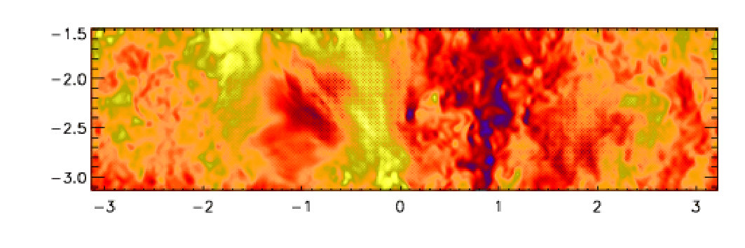
Fig. 2.3 Example of a velocity slice from a run where the time step is too long. Note the spurious checkerboard modulation in places, for example near \(x=-0.5\) and \(-2.5<y<-1.5\). This is an example of a hyperviscous turbulence simulations with \(512^3\) meshpoints and a third order hyperviscosity of \(\nu_3=5\times10^{-12}\). Hyperviscosity is explained in the Appendix~:ref:high-freq-filters.

Timestepping is accomplished using the Runge-Kutta 2N scheme. Regarding details of this scheme see Sect.~:ref:S-2N-scheme.

2.5.13.2. The Runge-Kutta-Fehlberg time step

A fifth order Runge-Kutta-Fehlberg time stepping procedure is available. It is used mostly for chemistry application, often together with the double precision option. In order to make this work, you need to compile with

TIMESTEP  =   timestep_rkf

in src/Makefile.local. In addition, you must put itorder=5 in run.in. An example application is samples/1d-tests/H2_flamespeed (in H2_flamespeed/).

Attention

This procedure is still experimental.

2.5.14. Boundary conditions

2.5.14.1. Where to specify boundary conditions

In most tests that come with the PENCIL CODE, boundary conditions are set in run.in, which is a natural choice. However, this may lead to unexpected initial data written by start.x, since when you start the code (via start.csh), the boundary conditions are unknown and start.x will then fill the ghost zones assuming periodicity (the default boundary condition) in all three directions. These ghost data will never be used in a calculation, as run.x will apply the boundary conditions before using any ghost-zone values.

To avoid these periodic conditions in the initial snapshot, you can set the boundary conditions in start.in already. In this case, they will be inherited by run.x, unless you also explicitly set boundary conditions in run.in.

2.5.14.2. How to specify boundary conditions

Boundary conditions are implemented through three layers of ghost points on either boundary, which is quite a natural choice for an MPI code that uses ghost zones for representing values located on the neighboring processors anyway. The desired type of boundary condition is set through the parameters bc{x,y,z} in run.in; the nomenclature used is as follows. Set bc{x,y,z} to a sequence of letters like

bcx = 'p','p','p', 'p',  'p'

for periodic boundaries, or

bcz = 's','s','a','a2','c1:c2'

for non-periodic ones. Each element corresponds to one of the variables, which are those of the variables \(u_x\), \(u_y\), \(u_z\), \(\ln\rho\), \(s/c_p\), \(A_x\), \(A_y\), \(A_z\), \(\ln c\) that are actually used in this order. The following conditions are available:

• p – periodic boundary condition

• a – antisymmetric condition w.r.t. the boundary (vanishing value)

• s – symmetric condition w.r.t. the boundary (vanishing first derivative)

• a2 – antisymmetry w.r.t. the arbitrary value on the boundary (vanishing second derivative)

• c1 – constant heat flux through the boundary (for \(\ln\rho\) and \(s\))

• c2 – constant temperature at the boundary (for \(s\); requires a2 for \(\ln\rho\))

• cT – constant temperature at the boundary (for arbitrarily set \(\ln\rho\))

• ce – set ghost-point temperature equal to boundary value (for arbitrarily set \(\ln\rho\))

• db – low-order one-sided derivatives (“no boundary condition”) for density

• she – shearing-sheet boundary condition (default when Shear is used)

• g – force boundary field values (requires force_lower_bound and force_upper_bound in init_pars)

• hs – enforce hydrostatic equilibrium at vertical boundaries (for \(\ln\rho\) and \(s\))

The extended syntax a:b (e.g. c1:c2) means: use boundary condition a at the lower boundary, but b at the upper one.

If you build a new run.in from another one with a different number of variables (noentropy vs. entropy, for example), you must adjust the length of the arrays bcx to bcz. The advantage of this approach is that it is easy to replace all boundary conditions in one direction at once (e.g. make everything periodic, or switch off shearing-sheet conditions and use stress-free boundaries instead).

2.5.15. Restarting a simulation

When a run stops at the end of a simulation, you can just resubmit the job again, and it will start from the latest snapshot saved in data/proc*/var.dat. The value of the latest time is saved in a separate file, data/proc*/time.dat. On parallel machines it is possible that some (or just one) of the var.dat are corrupt; for example after a system crash. Check for file size and date, and restart from a good VARN file instead.

If you want to run on a different machine, you just need to copy the data/proc*/var.dat (and, just to be sure) data/proc*/time.dat) files into a new directory tree. You may also need the data/proc*/seed.dat files for the random number generator. The easiest way to get all these other files is to run start.csh again on the new machine (or in a new directory) and then to overwrite the data/proc*/var.dat files with the correct ones.

For restarting from runs that didn’t have magnetic fields, passive scalar fields, or test fields, see Sect. RestartingFromLessPhysics.

2.5.16. One- and two-dimensional runs

If you want to run two-dimensional problems, set the number of mesh points in one direction to unity, e.g., nygrid`=1 or :file:`nzgrid`=1 in :file:`cparam.local. Remember that the number of mesh points is still divisible by the number of processors. For 2D-runs, it is also possible to write only 2D-snapshots (i.e. VAR files written only in the considered (\(x\),:math:y) or (\(x\),:math:z) plane, with a size seven times smaller as we do not write the third unused direction). To do that, please add the logical flag lwrite_2d=T in the namelist init_pars in start.in.

Similarly, for one-dimensional problems, set, for example, nygrid=1 and nzgrid=1 in cparam.local. You can even do a zero-dimensional run, but then you better set dt (rather than cdt), because there is no Courant condition for the time step.

See 0d, 1d, 2d, and 3d tests with examples.

2.5.17. Visualization

2.5.17.1. Gnuplot

Simple visualization can easily be done using Gnuplot, an open-source plotting program suitable for two-dimensional plots.

For example, suppose you have the variables

---it-----t-------dt-------urms-----umax-----rhom-----ssm------dtc---

in time_series.dat and want to plot \(u_{\rm rms}(t)\). Just start gnuplot and type

gnuplot> plot "data/time_series.dat" using 2:4 with lines

If you work over a slow line and want to see both \(u_{\rm rms}(t)\) and \(u_{\rm max}(t)\), use ASCII graphics:

gnuplot> set term dump
gnuplot> set logscale y
gnuplot> plot "data/time_series.dat" using 2:4 title "urms", \
gnuplot>      "data/time_series.dat" using 2:5 title "umax"

2.5.17.2. Data explorer

DX (data explorer; http://www.opendx.org) is an open-source tool for visualization of three-dimensional data.

PENCIL CODE provides a few networks for DX. It is quite easy to read in a snapshot file from DX (the only tricky thing is the four extra bytes at the beginning of the file, representing a Fortran record marker), and whenever you run start.x, the code writes a file var.general that tells DX all it needs to know about the data structure.

As a starting point for developing your own DX programs or networks, you can use a few generic DX scripts provided in the directory dx/basic/. From the run directory, start DX with

unix> dx -edit $PENCIL_HOME/dx/basic/lnrho

to load the file dx/basic/lnrho.net, and execute it with Ctl-o or Execute -> Execute Once. You will see a set of iso-surfaces of logarithmic density. If the viewport does not fit to your data, you can reset it with Ctl-f. To rotate the object, drag the mouse over the Image window with the left or right mouse button pressed. Similar networks are provided for entropy (ss.net), velocity (uu.net) and magnetic field (bb.net).

When you expand these simple networks to much more elaborate ones, it is probably a good idea to separate the different tasks (like Importing and Selecting, visualizing velocity, visualizing entropy, and Rendering) onto separate pages through Edit -> Page.

Note

Currently, DX can only read in data files written by one single processor, so from a multi-processor run, you can only visualize one subregion at a time.

2.5.17.3. GDL

GDL, also known as Gnu Data Language is a free visualization package that can be found at http://gnudatalanguage.sourceforge.net/. It aims at replacing the very expensive IDL package (see IDL). For the way we use IDL for PENCIL CODE, compatibility is currently not completely sufficient, but you can use GDL for many of the visualization tasks. If you get spurious “Error opening file” messages, you can normally simply ignore them.

2.5.17.3.1. Setup

As of GDL 0.9 – at least the version packed with Ubuntu Jaunty (9.10) – you will need to add GDL’s examples/pro/ directory to your !PATH variable. So the first call after starting GDL should be

GDL> .run setup_gdl

2.5.17.3.2. Starting visualization

There are mainly two possibilities for visualization: using a simple GUI or loading the data with pc_read and work with it interactively. Please note that the GUI was written and tested only with IDL (see Visualization in IDL).

Here, the pc_read family of IDL routines to read the data is described. Try

GDL> pc_read

to get an overview.

To plot a time series, use

GDL> pc_read_ts, OBJECT=ts
GDL> help, ts, /STRUCT  ;; (to see which slots are available)
GDL> plot, ts.t, ts.umax
GDL> oplot, ts.t, ts.urms

Alternatively, you could simply use the ts.pro script:

GDL> .run ts

To work with data from var.dat and similar snapshot files, you can e.g., use the following routines:

GDL> pc_read_dim, OBJECT=dim
GDL> $$PENCIL_HOME/bin/nl2idl -d ./data/param.nml> ./param.pro
GDL> pc_read_param, OBJECT=par
GDL> pc_read_grid, OBJECT=grid
GDL> pc_read_var, OBJECT=var

Having thus read the data structures, we can have a look at them to see what information is available:

GDL> help, dim, /STRUCT
GDL> help, par, /STRUCT
GDL> help, grid, /STRUCT
GDL> help, var, /STRUCT

To visualize data, we can e.g., do [10] :

GDL> plot, grid.x, var.ss[*, dim.ny/2, dim.nz/2]
GDL> contourfill, var.ss[*, *, dim.nz/2], grid.x, grid.y

GDL> ux_slice = var.uu[*, *, dim.nz/2, 0]
GDL> uy_slice = var.uu[*, *, dim.nz/2, 1]
GDL> wdvelovect, ux_slice, uy_slice, grid.x, grid.y

GDL> surface, var.lnrho[*, *, dim.nz/2, 0]

[10]

If contourfill produces just contour lines instead of a color-coded plot, your version of GDL is too old. E.g. the version shipped with Ubuntu 9.10 is based on GDL 0.9rc1 and has this problem.

See also Sect. IDL.

2.5.17.4. IDL

IDL is a commercial visualization program for two-dimensional and simple three-dimensional graphics. It allows to access and manipulate numerical data in a fashion quite similar to how Fortran handles them.

In $PENCIL_HOME/idl we provide a number of general-purpose IDL scripts that we are using all the time in connection with PENCIL CODE. While IDL is quite an expensive software package, it is quite useful for visualizing results from numerical simulations. In fact, for many applications, the 7-minute demo version of IDL is sufficient.

2.5.17.4.1. Visualization in IDL

The Pencil Code GUI is a data post-processing tool for the usage on a day-to-day basis. It allows fast inspection of many physical quantities, as well as advanced features like horizontal averages, streamline tracing, freely orientable 2D-slices, and extraction of cut images and movies. To use the Pencil Code GUI, it is sufficient to run:

unix> idl
IDL>  .r pc_gui

If you like to load only some subvolume of the data, like any 2D-slices from the given data snapshots, or 3D-subvolumes, it is possible to choose the corresponding options in the file selector dialog. The Pencil Code GUI offers also some options to be set on the command-line, please refer to their description in the source code.

There are also other small GUIs available, e.g., the file time-series.dat can easily be analyzed with the command:

unix> idl
IDL>  pc_show_ts

The easiest way to derive physical quantities at the command-line is to use one of the many pc_read_var-variants (pc_read_var_raw is recommended for large datasets because of its high efficiency regarding computation and memory usage) for reading the data. With that, one can make use of pc_get_quantity to derive any implemented physical quantity. Packed in a script, this is the recommended way to get reproducible results, without any chance for accidental errors on the interactive IDL command-line.

Alternatively, by using the command-line to see the time evolution of e.g., velocity and magnetic field (if they are present in your run), start IDL and run ts.pro:

unix> idl
IDL>  .run ts

The IDL script ts.pro script reads the time series data from data/time_series.dat and sorts the column into the structure ts, with the slot names corresponding to the name of the variables (taken from the header line of time_series.dat). Thus, you can refer to time as ts.t, to the rms velocity as ts.urms, and in order to plot the mean density as a function of time, you would simply type:

IDL> plot, ts.t, ts.rhom

The basic command sequence for working with a snapshot is:

unix> idl
IDL>  .run start
IDL>  .run r
IDL>  [specific commands] \

You run start.pro once to initialize (or reinitialize, if the mesh size has changed, for example) the fields and read in the startup parameters from the code. To read in a new snapshot, run r.pro (or rall.pro, see below).

If you are running in parallel on several processors, the data are scattered over different directories. To reassemble everything in IDL, use:

IDL> .r rall

instead of .r r (here, .r is a shorthand for .run). The procedure rall.pro reads (and assembles) the data from all processors and correspondingly requires large amounts of memory for very large runs. If you want to look at just the data from one processor, use r.pro instead.

If you need the magnetic field or the current density, you can calculate them in IDL by:

IDL> bb=curl(aa)
IDL> jj=curl2(aa)

By default one is reading always the current snapshot data/proc$N$/var.dat; if you want to read one of the permanent snapshots, use (for example):

IDL> varfile='VAR2'
IDL> .r r  (or .r rall)

With r.pro, you can switch the part of the domain by changing the variable datadir:

IDL> datadir='data/proc3'
IDL> .r r

will read the data written by processor 3.

Note

If you run IDL from the command line, you will highly appreciate the following tip: IDL’s command line editing is broken beyond hope. But you can fix it, by running IDL under rlwrap, a wrapper for the excellent GNU readline library. Download and install rlwrap from http://utopia.knoware.nl/~hlub/uck/rlwrap/ (on some systems you just need to run emerge rlwrap, or apt-get install rlwrap), and alias your idl command:

alias idl 'rlwrap -a -c idl'`` (csh)
alias idl='rlwrap -a -c idl'`` (bash)

From now on, you can

• use long command lines that correctly wrap around;

• type the first letters of a command and then PageUp to recall commands starting with these letters;

• capitalize, uppercase or lowercase a word with Esc-C, Esc-U, Esc-L;

• use command history across IDL sessions;

• complete file names with Tab;

• and use all other readline features that you are using in bash, octave, bc, gnuplot, ftp, etc.

2.5.17.4.2. Reading data into IDL arrays or structures

As an alternative to the method described above, there is also the possibility to read the data into structures. This makes some more operations possible, e.g., reading data from an IDL program where the command .r is not allowed.

IDL> pc_read_var_raw, obj=var, tags=tags
IDL> bb = pc_get_quantity ('B', var, tags)
IDL> jj = pc_get_quantity ('j', var, tags)

To read a snapshot VAR10 into the IDL structure ff, type:

IDL> pc_read_var, obj=ff, varfile='VAR10', /trimall

The option /trimall removes ghost zones from the data. You can see what data the structure contains by using the command tag_names:

IDL> print, tag_names(ff)
T X Y Z DX DY DZ UU LNRHO AA

One can access the individual variables by typing ff.varname, e.g.,

IDL> help, ff.aa
<Expression>    FLOAT     = Array[32, 32, 32, 3]

There are a number of files that read different data into structures. They are placed in the directory $PENCIL_HOME/idl/files contains files to read different data into structures, e.g.,

• pc_read_var_raw, obj=var, tags=tags

  Efficiently read a snapshot into an array.

• pc_read_var, obj=ff, /trimall

  Read a snapshot into a structure.

• pc_read_ts, obj=ts

  Read the time series into a structure.

• pc_read_xyaver, obj=xya ; pc_read_xzaver, obj=xza ; pc_read_yzaver, obj=yza

  Read 1-D time series into a structure.

• pc_read_const, obj=cst

  Read code constants into a structure.

• pc_read_pvar, obj=fp

  Read particle data into a structure.

• pc_read_param, obj=par

  Read startup parameters into a structure.

• pc_read_param, obj=par2, /param2

  Read runtime parameters into a structure.

Other options are documented in the source code of the files.

For examples on how to use these routines, see GDL.

2.5.17.5. Python

The PENCIL CODE supports reading, processing and the visualization of data using python. A number of scripts are placed in the subfolder $PENCIL_HOME/python. A README file placed under that subfolder contains the information needed to read Pencil output data into python.

2.5.17.5.1. Installation

For modern operating systems, Python is generally installed together with the system. If not, it can be installed via your preferred package manager or downloaded from the website https://www.python.org/. For convenience, it is strongly recommend to also install IPython, which is a more convenient console for Python. You will also need the Python packages NumPy, matplotlib, h5py, Tk and often Dill.

Perhaps the easiest way to obtain all the required software mentioned above is to install either Continuum’s Anaconda or Enthought’s Canopy. These Python distributions also provide (or indeed are) integrated graphical development environments.

Another way of installing libraries, particularly on a cluster without root privileges, is to use pip or pip3: pip install h5py or pip3 install h5py.

In order for Python to find the Pencil Code commands, you will have to set the environment variable PYTHONPATH:

export PYTHONPATH=${PENCIL_HOME}/python
# or
export PYTHONPATH=${PENCIL_HOME}/python:${PYTHONPATH}

Normally, you will add one of these lines to your .bashrc file.

In addition, you have to import the pencil module each time you start a Python shell:

import pencil as pc

The next two paragraphs show how you can include this and some other imports into your Python interpreter setup, so they are automatically run when you start IPython or the Python REPL.

2.5.17.5.2. ipythonrc

When using IPython, some Pencil Code users add the following line to their .ipython/ipythonrc (create the file if it doesn’t exist):

import_all pencil

and in addition add to their .ipython/profile_default/startup/init.py the lines:

import pencil as pc

import numpy as np
import pylab as plt
import matplotlib
from matplotlib import rc

plt.ion()
matplotlib.rcParams['savefig.directory'] = ''

2.5.17.5.3. .pythonrc

If you don’t have IPython and cannot install it (e.g., on some cluster), you can instead edit your .pythonrc:

#!/usr/bin/python
import numpy as np
import pylab as plt
import pencil as pc
import atexit
#import readline
import rlcompleter

# enables search with Ctrl+r in the history
try:
    import readline
except ImportError:
    print "Module readline not available."
else:
    import rlcompleter
    readline.parse_and_bind("tab: complete")
# enables command history
historyPath = os.path.expanduser("~/.pyhistory")
def save_history(historyPath=historyPath):
    import readline
    readline.write_history_file(historyPath)
if os.path.exists(historyPath):
    readline.read_history_file(historyPath)
atexit.register(save_history)
del os, atexit, readline, rlcompleter, save_history, historyPath

plt.ion()

and create the file .pythonhistory and add to your .bashrc:

export PYTHONSTARTUP=~/.pythonrc

However, none of this is required to use the Pencil Code Python modules.

2.5.17.5.4. Pencil Code Commands in General

For a list of all Pencil Code commands start IPython and type pc. <TAB> (as with auto completion). To access the help of any command just type the command followed by a ‘?’ (no spaces), e.g.,

In [1]: pc.math.dot?
Signature: pc.math.dot(a, b)
Docstring:
Take dot product of two pencil-code vectors a and b.

call signature:

dot(a, b):

Keyword arguments:

*a*, *b*:
  Pencil-code vectors with shape [3, mz, my, mx].
File:      ~/pencil-code/python/pencil/math/vector_multiplication.py
Type:      function

You can also use help(pc.dot) for a more complete documentation of the command.

There are various reading routines for the Pencil Code data. All of them return an object with the data. To store the data into a user defined variable type, e.g.,

In [1]: ts = pc.read.ts()

Most commands take some arguments. For most of them there is a default value, e.g.,

In [1]: pc.read.ts(file_name='time_series.dat', datadir='data')

2.5.17.5.5. Reading and Plotting Time Series

Reading the time series file is very easy. Simply type

In [1]: ts = pc.read.ts()

and Python stores the data in the variable ts. The physical quantities are members of the object ts and can be accessed accordingly, e.g., ts.t, ts.emag. To check which other variables are stored simply do the tab auto completion ts. <TAB>.

Plot the data with the matplotlib commands:

In [1]: plt.plot(ts.t, ts.emag)

The standard plots are not perfect and need a little polishing. See the online wiki for a few examples on how to make pretty plots (https://github.com/pencil-code/pencil-code/wiki/PythonForPencil). You can save the plot into a file using the GUI or with

In [1]: plt.savefig('plot.eps')

2.5.17.5.6. Reading and Plotting VAR files and slice files

Read var files:

In [1]: var = pc.read.var()

Read slice files:

In [1]: slices = pc.read.slices(field='bb1', extension='xy')

This returns the object slices with indices slices[nTimes, my, mx] and the time array t.

If you want to plot, e.g., the x-component of the magnetic field at the central plane simply type:

In [1]: plt.imshow(var.bb[0, 128, :, :].T, origin='lower', extent=[-4, 4, -4, 4])

For a complete list of arguments of plt.imshow refer to its documentation.

For a more interactive plot use:

In [1]: pc.visu.animate_interactive(slices.xy.bb1, t)

Be aware

arrays from the reading routines are ordered f[nvar, mz, my, mx], i.e. reversed to IDL. This affects reading var files and slice files.

2.5.18. Running on multi-processor computers

The code is parallelized using MPI for a simple domain decomposition (data-parallelism), which is a straight-forward and very efficient way of parallelizing finite-difference codes. The current version has a few restrictions, which need to be kept in mind when using the MPI features.

The global number of grid points (but excluding the ghost zones) in a given direction must be an exact multiple of the number of processors you use in that direction. For example if you have nprocy=8 processors for the \(y\) direction, you can run a job with nygrid=64 points in that direction, but if you try to run a problem with nygrid=65 or nygrid=94, the code will complain about an inconsistency and stop. (So far, this has not been a serious restriction for us.)

2.5.18.1. How to run a sample problem in parallel

To run the sample problem in the directory samples/conv-slab on 16 CPUs, you need to do the following (in that directory):

1. Edit src/Makefile.local and replace

   MPICOMM   = nompicomm \
   

   by

   MPICOMM   =   mpicomm \
   

2. Edit src/cparam.local and replace

   integer, parameter :: ncpus=1, nprocy=1, nprocz=ncpus/nprocy, nprocx=1
   integer, parameter :: nxgrid=32, nygrid=nxgrid, nzgrid=nxgrid \
   

   by

   integer, parameter :: ncpus=16, nprocy=4, nprocz=ncpus/nprocy, nprocx=1
   integer, parameter :: nxgrid=128, nygrid=nxgrid, nzgrid=nxgrid \
   

   The first line specifies a \(4{\times}4\) layout of the data in the \(y\) and \(z\) direction. The second line increases the resolution of the run because running a problem as small as \(32^3\) on 16 CPUs would be wasteful. Even \(128^3\) may still be quite small in that respect. For performance timings, one should try and keep the size of the problem per CPU the same, so for example \(256^3\) on 16 CPUs should be compared with \(128^3\) on 2 CPUs.

3. Recompile the code

   unix> (cd src; make)
   

4. Run it

   unix> start.csh
   unix> run.csh
   

Make sure that all CPUs see the same data/ directory; otherwise things will go wrong.

Remember that in order to visualize the full domain with IDL (rather than just the domain processed and written by one processor), you need to use rall.pro instead of r.pro.

2.5.18.2. Hierarchical networks (e.g., on Beowulf clusters)

On big Beowulf clusters, a group of nodes is often connected with a switch of modest speed, and all these groups are connected via a \(n\) times faster uplink switch. When bandwidth-limited, it is important to make sure that consecutive processors are mapped onto the mesh such that the load on the uplink is \(\lesssim n\) times larger than the load on the slower switch within each group. On a 512 node cluster, where groups of 24 processors are linked via fast ethernet switches, which in turn are connected via a Gigabit uplink (\(\sim 10\) times faster), we found that nprocy=4 is optimal. For 128 processors, for example we find that \(nprocy \times nprocz=4\times32\) is the optimal layout. For comparison, \(8\times16\) is 3 times slower, and \(16\times8\) is 17 (!) times slower. These results can be understood from the structure of the network, but the basic message is to watch out for such effects and to try varying nprocy and nprocz.

In cases where nygrid > nzgrid it may be advantageous to swap the ordering of processor numbers. This can be done by setting lprocz_slowest = F.

2.5.18.3. Extra workload caused by the ghost zones

Normally, the workload caused by the ghost zones is negligible. However, if one increases the number of processors, a significant fraction of work is done in the ghost zones. In other words, the effective mesh size becomes much larger than the actual mesh size.

Consider a mesh of size \(N_w=N_x\times N_y\times N_z\), and distribute the task over \(P_w=P_x\times P_y\times P_z\) processors. If no communication were required, the number of points per processor would be

\[{N_w\over P_w}={N_x\times N_y\times N_z\over P_x\times P_y\times P_z}.\]

However, for finite difference codes some communication is required, and the amount of communication depends on spatial order of the scheme, \(Q\). The PENCIL CODE works by default with sixth order finite differences, so \(Q=6\), i.e., one needs 6 ghost zones, 3 on each end of the mesh. With \(Q\neq0\) the number of points per processor is

\[{N_w^{\rm(eff)}\over P_w}= \left({N_x\over P_x}+Q\right)\times \left({N_y\over P_y}+Q\right)\times \left({N_z\over P_z}+Q\right).\]

There is efficient scaling only when

\[\min\left({N_x\over P_x}, {N_y\over P_y}, {N_z\over P_z}\right)\gg Q.\]

In the special case where \(N_x=N_y=N_z\equiv N=N_w^{1/3}\), with \(P_x=1\) and \(P_y=P_z\equiv P=P_w^{1/2}\), we have

\[{N_w^{\rm(eff)}\over P_w}= \left(N+Q\right)\times \left({N\over P}+Q\right)^2.\]

For \(N=128\) and \(Q=6\) the effective mesh size exceeds the actual mesh size by a factor

\[{N_w^{\rm(eff)}\over N_w} =\left(N+Q\right)\times\left({N\over P}+Q\right)^2\times{P_w\over N_w}.\]

These factors are listed in Table 2.3.

Table 2.3 \(N_w^{\rm(eff)}/N_w\) versus \(N\) and \(P\).

P N	128	256	512	1024	2048
1	1.15	1.07	1.04	1.02	1.01
2	1.19	1.09	1.05	1.02	1.01
4	1.25	1.12	1.06	1.03	1.01
8	1.34	1.16	1.08	1.04	1.02
16	1.48	1.22	1.11	1.05	1.03
32	1.68	1.31	1.15	1.07	1.04
64	1.98	1.44	1.21	1.10	1.05
128	2.45	1.64	1.30	1.14	1.07
256	3.21	1.93	1.43	1.20	1.10
512	4.45	2.40	1.62	1.29	1.14

Ideally, one wants to keep the work in the ghost zones at a minimum. If one accepts that 20–25% of work are done in the ghost zones, one should use 4 processors for \(128^3\) mesh points, 16 processors for \(256^3\) mesh points, 64 processors for \(512^3\) mesh points, 256 processors for \(1024^3\) mesh points, and 512 processors for \(1536^3\) mesh points.

2.5.19. Running in double-precision

With many compilers, you can easily switch to double precision (8-byte floating point numbers) as follows.

Add the lines

# Use double precision
REAL_PRECISION = double

to src/Makefile.local and (re-)run pc_setupsrc.

If REAL_PRECISION is set to double, the flag FFLAGS_DOUBLE is appended to the Fortran compile flags. The default for FFLAGS_DOUBLE is -r8, which works for g95 or ifort; for gfortran, you need to make sure that FFLAGS_DOUBLE is set to -fdefault-real-8.

You can see the flags in src/Makefile.inc, which is the first place to check if you have problems compiling for double precision.

medskip

Using double precision might be important in turbulence runs where the resolution is \(256^3\) meshpoints and above (although such runs often seem to work fine at single precision).

To continue working in double precision, you just say lread_from_other_prec=T in run_pars; see After-changing-REALPRECISION.

2.5.20. Power spectrum

Given a real variable \(u\), its Fourier transform \(\tilde{u}\) is given by

\[\tilde{u}(k_x,k_y,k_z) \ =\ \mathcal{F}(u(x,y,z)) = \frac{1}{N_x N_y N_z} \sum_{p=0}^{N_x-1} \sum_{q=0}^{N_y-1} \sum_{r=0}^{N_z-1} u(x_p,y_q,z_r) \exp(-i k_x x_p) \exp(-i k_y y_q) \exp(-i k_z z_r) ,\]

where

\[|k_x| < \frac{\pi N_x}{L_x} \, ,\qquad |k_y| < \frac{\pi N_y}{L_y} \, ,\qquad |k_z| < \frac{\pi N_z}{L_z} \, ,\]

when \(L\) is the size of the simulation box. The three-dimensional power spectrum \(P(k)\) is defined as

\[P(k)=\frac{1}{2}\tilde{u}\tilde{u}^*,\]

where

\[k=\sqrt{k_x^2+k_y^2+k_z^2} .\]

Note that we can only reasonably calculate \(P(k)\) for \(k < \pi N_x/L_x\).

To get power spectra from the code, edit run.in and add for example the following lines

dspec=5., ou_spec=T, ab_spec=T !(for energy spectra)
oned=T

under run_pars. The kinetic (vel_spec) and magnetic (mag_spec) power spectra will now be calculated every 5.0 (dspec) time units. The Fourier spectra is calculated using fftpack. In addition to calculating the three-dimensional power spectra also the one-dimensional power spectra will be calculated (oned).

In addition one must edit src/Makefile.local and add the lines

FOURIER = fourier_fftpack
POWER = power_spectrum

Running the code will now create the files powerhel_mag.dat and power_kin.dat containing the three-dimensional magnetic and kinetic power spectra respectively. In addition to these three-dimensional files we will also find the one-dimensional files powerbx_x.dat, powerby_x.dat, powerbz_x.dat, powerux_x.dat, poweruy_x.dat and poweruz_x.dat. In these files the data are stored such that the first line contains the time of the snapshot, the following nxgrid/2 numbers represent the power at each wavenumber, from the smallest to the largest. If several snapshots have been saved, they are being stored immediately following the preceding snapshot.

You can read the results with the idl procure power, like this:

power,'_kin','_mag',k=k,spec1=spec1,spec2=spec2,i=n,tt=t,/noplot
power,'hel_kin','hel_mag',k=k,spec1=spec1h,spec2=spec2h,i=n,tt=t,/noplot

If powerhel is invoked, krms is written during the first computation. The relevant output file is power_krms.dat. This is needed for a correct calculation of \(k\) used in the realizability conditions.

A caveat of the implementation of Fourier transforms in the Pencil Code is that, due to the parallelization, the permitted resolution is limited to the case when one direction is an integer multiple of the other. So, it can be done for

Nx = n*Ny

Unfortunately, for some applications one wants Nx < Ny. Wlad experimented with arbitrary resolution by interpolating \(x\) to the same resolution of \(y\) prior to transposing, then transform the interpolated array and then interpolating it back (check fourier_transform_y in fourier_fftpack.f90).

A feature of our current implementation with \(x\) parallelization is that fft_xyz_parallel_3D requires nygrid to be an integer multiple of nprocy*nprocz. Examples of good mesh layouts are listed in Table 2.4.

Table 2.4 Examples of mesh layouts for which Fourier transforms with \(x\) parallelization is possible.

ny	nprocx	nprocy	nprocz	ncpus
256	1	16	16	256
256	2	16	16	512
256	4	16	16	1024
256	8	16	16	2048
288	2	16	18	576
512	2	16	32	1024
512	4	16	16	1024
512	4	16	32	2048
576	4	18	32	2304
576	8	18	32	4608
576	16	18	32	9216
1024	4	32	32	4096
1024	4	16	64	4096
1024	8	16	32	4096
1152	4	36	32	4608
1152	4	32	36	4608
2304	2	32	72	4608
2304	4	36	64	9216
2304	4	32	72	9216

To visualize with IDL just type power and you get the last snapshot of the three-dimensional power spectrum. See head of $PENCIL_HOME/idl/power.pro for options to power.

By default, the spectra for the initial times time is not outputted, but it can sometimes be useful to have it. In that case, one can put lspec_start=T.

2.5.21. Other power spectra

Over the years, many more spectra have been outputted and not everything is immediately documented. Here some examples:

data/powerhel_mag.dat
data/powerhel_kin.dat
data/power_saffman_ub.dat
data/power_saffman_mag.dat
data/power_mag.dat
data/power_krms.dat
data/power_kin.dat

Here, the first two are helicity spectra that come for free (in addition to those with _kin and _mag) when one invokes ou_spec=T and ab_spec=T. The ones with _saffman refer to the spectra related to Saffman-like invariants such as the Hosking integral (which refers to power_mag.dat) and the cross-helicity Saffman-like invariant (power_saffman_ub.dat). Their slopes for \(k\to0\) are the invariants divided by \(2\pi^2\); see the papers by Hosking & Schekochihin (2021) as well as Zhou et al. (2022).

2.5.22. Structure functions

We define the p-th order longitudinal structure function of \(\vec{u}\) as

\[S^p_{\rm long}(l)=\left< | u_x(x{+}l,y,z)-u_x(x,y,z)|^p \right> \; ,\]

while the transverse is

\[S^p_{\rm trans}(l)= \left< | u_y(x{+}l,y,z)-u_y(x,y,z)|^p \right> + \left< | u_z(x{+}l,y,z)-u_z(x,y,z)|^p \right> \; .\]

Edit run.in and add for example the following lines

dspec=2.3,
lsfu=T, lsfb=T, lsfz1=T, lsfz2=T

under run_pars. The velocity (lsfu), magnetic (lsfb) and Elsasser (lsfz1 and lsfz2) structure functions will now be calculated every 2.3 (dspec) time unit.

In addition one must edit src/Makefile.local and add the line

STRUCT_FUNC = struct_func

In src/cparam.local, define lb_nxgrid and make sure that

nxgrid = nygrid = nzgrid = 2**lb_nxgrid

E.g.

integer, parameter :: lb_nxgrid=5
integer, parameter :: nxgrid=2**lb_nxgrid,nygrid=nxgrid,nzgrid=nxgrid

Running the code will now create the files:

• sfu-1.dat, sfu-2.dat, sfu-3.dat (velocity),

• sfb-1.dat, sfb-2.dat, sfb-3.dat (magnetic field),

• sfz1-1.dat, sfz1-2.dat, sfz1-3.dat (first Elsasser variable),

• sfz2-1.dat, sfz2-2.dat, sfz2-3.dat (second Elsasser variable),

which contains the data of interest. The first line in each file contains the time \(t\) and the number qmax, such that the largest moment calculated is qmax-1. The next imax numbers represent the first moment structure function for the first snapshot, here

\[imax=2\frac{\ln (nxgrid)}{\ln 2}-2.\]

The next imax numbers contain the second moment structure function, and so on until qmax-1. The following imax numbers then contain the data of the signed third order structure function i.e. \(S^3_{\rm long}(l)=\left< [u_x(x{+}l,y,z)-u_x(x,y,z)]^3 \right>\).

The following imax × qmax × 2 numbers are zero if nr_directions=1 (default), otherwise they are the same data as above but for the structure functions calculated in the y and z directions.

If the code has been run long enough as to calculate several snapshots, these snapshots will now follow, being stored in the same way as the first snapshot.

To visualize with IDL just type structure and you get the time-average of the first order longitudinal structure function (be sure that pencil-runs/forced/idl/ is in IDL_PATH). See head of pencil-runs/forced/idl/structure.pro for options to structure.

2.5.23. Particles

The PENCIL CODE has modules for tracer particles and for dust particles (see Sect. Particles). The particle modules are chosen by setting the value of the variable PARTICLES in Makefile.local to either particles_dust or particles_tracers. For the former case each particle has six degrees of freedom, three positions and three velocities. For the latter it suffices to have only three position variables as the velocity of the particles are equal to the instantaneous fluid velocity at that point. In addition one can choose to have several additional internal degrees of freedoms for the particles. For example one can temporally evolve the particles radius by setting PARTICLES_RADIUS to particles_radius in Makefile.local.

All particle infrastructure is controlled and organized by the Particles_main module. This module is automatically selected by Makefile.src if PARTICLES is different from noparticles. Particle modules are compiled as a separate library. This way the main part of the PENCIL CODE only needs to know about the particles_main.a library, but not of the individual particle modules.

For a simulation with particles one must in addition define a few parameters in cparam.local. Here is a sample of cparam.local for a parallel run with 2,000,000 particles:

integer, parameter :: ncpus=16, nprocy=4, nprocz=4, nprocx=1
integer, parameter :: nxgrid=128, nygrid=256, nzgrid=128
integer, parameter :: npar=2000000, mpar_loc=400000, npar_mig=1000
integer, parameter :: npar_species=2

The parameter npar is the number of particles in the simulation, mpar_loc is the number of particles that is allowed on each processor and npar_mig is the number of particles that are allowed to migrate from one processor to another in any time-step. For a non-parallel run it is enough to specify npar. The number of particle species is set through npar_species (assumed to be one if not set). The particle input parameters are given in start.in and run.in. Here is a sample of the particle part of start.in for dust particles:

/
&particles_init_pars
  initxxp='gaussian-z', initvvp='random'
  zp0=0.02, delta_vp0=0.01, eps_dtog=0.01, tausp=0.1
  lparticlemesh_tsc=T
/

The initial positions and velocities of the dust particles are set in initxxp and initvvp. The next four input parameters are further specifications of the initial condition. Interaction between the particles and the mesh, e.g., through drag force or self-gravity, require a mapping of the particles on the mesh. The PENCIL CODE currently supports NGP (Nearest Grid Point, default), CIC (Cloud in Cell, set lparticlemesh_cic=T) and TSC (Triangular Shaped Cloud, set lparticlemesh_tsc=T). See Youdin & Johansen (2007) for details.

Here is a sample of the particle part of run.in (also for dust particles):

/
&particles_run_pars
  ldragforce_gas_par=T
  cdtp=0.2
/

The logical ldragforce_gas_par determines whether the dust particles influence the gas with a drag force. cdtp tells the code how many friction times should be resolved in a minimum time-step.

The sample run samples/sedimentation/ contains the latest setup for dust particles.

2.5.23.1. Particles in parallel

The particle variables (e.g., \(\vec{x}_i\) and \(\vec{v}_i\)) are kept in the arrays fp and dfp. For parallel runs, particles must be able to move from processor to processor as they pass out of the \((x,y,z)\)-interval of the local processor. Since not all particles are present at the same processor at the same time (hopefully), there is some memory optimization in making fp not big enough to contain all the particles at once. This is achieved by setting the code variable mpar_loc less than npar in cparam.local for parallel runs. When running with millions of particles, this trick is necessary to keep the memory need of the code down.

The communication of migrating particles between the processors happens as follows (see the subroutine redist_particles_procs in particles_sub.f90):

1. In the beginning of each time-step all processors check if any of their particles have crossed the local \((x,y,z)\)-interval. These particles are called migrating particles. A run can have a maximum of npar_mig migrating particles in each time-step. The value of npar_mig must be set in cparam.local. The number should (of course) be slightly larger than the maximum number of migrating particles at any time-step during the run. The diagnostic variable nmigmax can be used to output the maximum number of migrating particles at a given time-step. One can set lmigration_redo=T in &particles_run_pars to force the code to redo the migration step if more than npar_mig want to migrate. This does slow the code down somewhat, but has the benefit that the code does not stop when more than npar_mig particles want to migrate.

2. The index number of the receiving processor is then calculated. This requires some assumption about the grid on other processors and will currently not work for nonequidistant grids. Particles do not always pass to neighboring processors as the global boundary conditions may send them to the other side of the global domains (periodic or shear periodic boundary conditions).

3. The migrating particle information is copied to the end of fp, and the empty spot left behind is filled up with the particle of the highest index number currently present at the processor.

4. Once the number of migrating particles is known, this information is shared with neighboring processors (including neighbors over periodic boundaries) so that they all know how many particles they have to receive and from which processors.

5. The communication happens as directed MPI communication. That means that processors 0 and 1 can share migrating particles at the same time as processors 2 and 3 do it. The communication happens from a chunk at the end of fp (migrating particles) to a chunk that is present just after the particle of the highest index number that is currently at the receiving processor. Thus the particles are put directly at their final destination, and the migrating particle information at the source processor is simply overwritten by other migrating particles at the next time-step.

6. Each processor keeps track of the number of particles that it is responsible for. This number is stored in the variable npar_loc. It must never be larger than mpar_loc (see above). When a particle leaves a processor, npar_loc is reduced by one, and then increased by one at the processor that receives that particle. The maximum number of particles at any processor is stored in the diagnostic variable nparmax. If this value is not close to npar/ncpus, the particles have piled up in such a way that computations are not evenly shared between the processors. One can then try to change the parallelization architecture (nprocy and nprocz) to avoid this problem.

In simulations with many particles (comparable to or more than the number of grid cells), it is crucial that particles are shared relatively evenly among the processors. One can as a first approach attempt to not parallelize directions with strong particle density variations. However, this is often not enough, especially if particles clump locally.

Alternatively one can use Particle Block Domain Decomposition (PBDD, see Johansen et al. 2011). The steps in Particle Block Domain Decomposition scheme are as follows:

1. The fixed mesh points are domain-decomposed in the usual way (with ncpus = nprocx * nprocy * nprocz).

2. Particles on each processor are counted in bricks of size nbx * nby * nbz (typically nbx = nby = nbz = 4).

3. Bricks are distributed among the processors so that each processor has approximately the same number of particles.

4. Adopted bricks are referred to as blocks.

5. The PENCIL CODE uses a third order Runge-Kutta time-stepping scheme. In the beginning of each sub-time-step particles are counted in blocks and the block counts communicated to the bricks on the parent processors. The particle density assigned to ghost cells is folded across the grid, and the final particle density (defined on the bricks) is communicated back to the adopted blocks. This step is necessary because the drag force time-step depends on the particle density, and each particle assigns density not just to the nearest grid point, but also to the neighboring grid points.

6. In the beginning of each sub-time-step the gas density and gas velocity field is communicated from the main grid to the adopted particle blocks.

7. Drag forces are added to particles and back to the gas grid points in the adopted blocks. This partition aims at load balancing the calculation of drag forces.

8. At the end of each sub-time-step the drag force contribution to the gas velocity field is communicated from the adopted blocks back to the main grid.

Particle Block Domain Decomposition is activated by setting PARTICLES = particles_dust_blocks and PARTICLES_MAP = particles_map_blocks in Makefile.local. A sample of cparam.local for Particle Block Domain Decomposition can be found in samples/sedimentation/blocks:

integer, parameter :: ncpus=4, nprocx=2, nprocy=2, nprocz=1
integer, parameter :: nxgrid=32, nygrid=32, nzgrid=32
integer, parameter :: npar=10000, mpar_loc=5000, npar_mig=100
integer, parameter :: npar_species=4
integer, parameter :: nbrickx=4, nbricky=4, nbrickz=4, nblockmax=32

The last line defines the number of bricks in the total domain – here we divide the grid into 4 x 4 x 4 bricks each of size 8 x 8 x 8 grid points. The parameter nblockmax tells the code the maximum number of blocks any processor may adopt. This should not be so low that there is not room for all the bricks with particles, nor so high that the code runs out of memory.

2.5.23.2. Large number of particles

When dealing with large number of particles, one needs to make sure that the number of particles npar is less than the maximum integer that the compiler can handle with. The maximum integer can be checked by the Fortran intrinsic function huge:

program huge_integers
  print *, huge(0_4) ! for default Fortran integer (32 Bit)
  print *, huge(0_8) ! for 64 Bit integer in Fortran
end program huge_integers

If the number of particles npar is larger than default maximum integer, one can promote the maximum integer to 64 Bit by setting:

integer(kind=8), parameter :: npar=4294967296

in the cparam.local file. This works because the data type of npar is only set here. It is worth noting that one should not use the flag:

FFLAGS += -integer-size 64

to promote all the integers to 64 Bit. This will break the Fortran-C interface. One should also make sure that npar_mig <= npar/ncpus. It is also beneficial to set mpar_loc = 2*npar/ncpus.

Sometimes one may encounter the following error, “additional relocation overflows omitted from the output” due to the 2G memory limit (caused by large static array). It is mpar_loc that determines the usage of memory instead of npar. There are two ways to resolve this issue:

• Use a specific memory model to generate code and store data by setting the

  following for Intel compiler in your configuration file:

  FFLAGS += -shared-intel -mcmodel=medium
  

  This will, however, affect the performance of the code. This method can handle at least the following setup:

  integer, parameter :: ncpus=256, nprocx=4, nprocy=8, nprocz=ncpus/(nprocx*nprocy)
  integer, parameter :: nxgrid=1024, nygrid=nxgrid, nzgrid=nxgrid
  integer(kind=ikind8), parameter :: npar=124999680
  integer, parameter :: npar_stalk=100000, npar_mig=npar/10
  integer, parameter :: mpar_loc=npar/5
  

• Increase ncpu and decrease mpar_loc. For

  npar=124999680, ncpu=1024 is needed.

  integer, parameter :: ncpus=1024, nprocx=8, nprocy=8, nprocz=ncpus/(nprocx*nprocy)
  integer, parameter :: nxgrid=1024, nygrid=nxgrid, nzgrid=nxgrid
  integer(kind=ikind8), parameter :: npar=124999680
  integer, parameter :: mpar_loc=5*npar/ncpus
  integer, parameter :: npar_stalk=100000, npar_mig=npar/ncpus
  

It is worth noting that even without particles, a simulation with 1024^3 resolution requires at least 512 CPUs to be compiled.

2.5.23.3. Random number generator

There are several methods to generate random number in the code. It is worth noting that when simulating coagulation with the super-particle approach, one should use the intrinsic random number generator of FORTRAN instead of the one implemented in the code. When invoking random_number_wrapper, there will be back-reaction to the gas flow. This unexpected back-reaction can be tracked by inspecting the power spectra, which exhibits the oscillation at the tail. To avoid this, one should set luser_random_number_wrapper=F under the module particles_coag_run_pars in run.in.

2.5.24. Non-cartesian coordinate systems

Spherical coordinates are invoked by adding the following line in the file start.in:

&init_pars
  coord_system='spherical_coords'

One can also invoke cylindrical coordinates by saying cylindrical_coords instead. In practice, the names \((x,y,z)\) are still used, but they then refer to \((r,\theta,\phi)\) or \((r,\phi,z)\) instead.

When working with curvilinear coordinates it is convenient to use differential operators in the non-coordinate basis, so the derivatives are taken with respect to length, and not in a mixed fashion with respect to length for \(\partial/\partial r\) and with respect to angle for \(\partial/\partial \theta\) and \(\partial/\partial \phi\). The components in the non-coordinate basis are denoted by hats, see, e.g., [MTW], p. 213; see also Appendix B of [MTBM09].

For spherical polar coordinates the only nonvanishing Christoffel symbols (or connection coefficients) are:

\[{\Gamma^{\hat\theta}}_{{\hat r}{\hat\theta}} ={\Gamma^{\hat\phi}}_{{\hat r}{\hat\phi}} =-{\Gamma^{\hat r}}_{{\hat\theta}{\hat\theta}} =-{\Gamma^{\hat r}}_{{\hat\phi}{\hat\phi}} =1/r,\]

\[{\Gamma^{\hat\phi}}_{{\hat\theta}{\hat\phi}} =-{\Gamma^{\hat\theta}}_{{\hat\phi}{\hat\phi}} =\cot\theta/r.\]

The Christoffel symbols enter as correction terms for the various differential operators in addition to a term calculated straightforwardly in the non-coordinate basis. The derivatives of some relevant Christoffel symbols are:

\[{\Gamma^{\hat\theta}}_{\hat r\hat\theta,\hat\theta} ={\Gamma^{\hat\phi}}_{\hat r\hat\phi,\hat\phi} ={\Gamma^{\hat\phi}}_{\hat\theta\hat\phi,\hat\phi}=0\]

\[{\Gamma^{\hat\theta}}_{\hat r\hat\theta,\hat r} ={\Gamma^{\hat\phi}}_{\hat r\hat\phi,\hat r}=-r^{-2}\]

\[{\Gamma^{\hat\phi}}_{\hat\theta\hat\phi,\hat\theta}=-r^{-2}\sin^{-2}\!\theta\]

Further details are given in Curvilinear-coordinates.

2.6. The equations

The equations solved by the PENCIL CODE are basically the standard compressible MHD equations. However, the modular structure allows some variations of the MHD equations, as well as switching off some of the equations or individual terms of the equation (nomagnetic, noentropy, etc.).

In this section the equations are presented in their most complete form. It may be expected that the code can evolve most subsets or simplifications of these equations.

2.6.1. Continuity equation

In the code the continuity equation, \(\partial\rho/\partial t + \nabla\cdot(\rho\mathbf{u}) = 0\), is written in terms of \(\ln\rho\),

(2.5)\[\frac{\De \ln\rho}{\De t} = - \Div \uv \; .\]

Here \(\rho\) denotes density, \(\uv\) the fluid velocity, \(t\) is time and \(\De/\De t \equiv \partial/\partial t + \mathbf{u}\cdot\nabla\) is the advective derivative.

2.6.2. Equation of motion

In the equation of motion, using a perfect gas, the pressure term, can be expressed as \(-\rho^{-1}\grad p = -\cs^2(\grad s/c_p+\grad\ln\rho)\), where the squared sound speed is given by

(2.6)\[\cs^2 = \gamma \frac{p}{\rho} = c_{\rm s0}^2\exp\left[\gamma s/c_p + (\gamma{-}1)\ln\frac{\rho}{\rho_0} \right],\]

and \(\gamma=c_p/c_v\) is the ratio of specific heats, or adiabatic index. Note that \(\cs^2\) is proportional to the temperature with \(\cs^2=(\gamma-1)c_p T\).

The equation of motion is accordingly

(2.7)\[\frac{\De\uv}{\De t} = -\cs^2\grad\biggl(\frac{s}{c_p} + \ln\rho\biggr) - \grad\Phi_{\rm grav} + \frac{\jv\times\Bv}{\rho} + \nu \left( \Laplace\uv + \frac{1}{3}\grad\Div\uv + 2\Strain\cdot\grad\ln\rho\right) + \zeta\left(\grad\Div\uv\right);\]

Here \(\Phi_{\rm grav}\) is the gravity potential, \(\jv\) the electric current density, \(\Bv\) the magnetic flux density, \(\nu\) is kinematic viscosity, \(\zeta\) describes a bulk viscosity, and, in Cartesian coordinates

(2.8)\[{\mathsf S}_{ij} = \frac{1}{2}\left({\partial u_i\over\partial x_j} + {\partial u_j\over\partial x_i} -\frac{2}{3} \delta_{ij}\Div\uv\right)\]

is the rate-of-shear tensor that is traceless, because it can be written as the generic rate-of-strain tensor minus its trace. In curvilinear coordinates, we have to replace partial differentiation by covariant differentiation (indicated by semicolons), so we write \({\mathsf S}_{ij}=\frac{1}{2}(u_{i;j}+u_{j;i})-\frac{1}{3}\delta_{ij}\Div\uv\).

The interpretation of the two viscosity terms varies greatly depending upon the Viscosity module used, and indeed on the parameters given to the module. See Bulkviscosity.

For isothermal hydrodynamics, see Entropy equation below.

2.6.3. Induction equation

(2.9)\[\frac{\partial\Av}{\partial t} = \uv\times\Bv - \eta\mu_0\jv \; .\]

Here \(\Av\) is the magnetic vector potential, \(\Bv\) = \(\boldsymbol{\nabla}\times\) \(\Av\) the magnetic flux density, \(\eta = 1/(\mu_0\sigma)\) is the magnetic diffusivity (\(\sigma\) denoting the electrical conductivity), and \(\mu_0\) the magnetic vacuum permeability. This form of the induction equation corresponds to the Weyl gauge \(\Phi=0\), where \(\Phi\) denotes the scalar potential.

2.6.4. Entropy equation

The current thermodynamics module entropy formulates the thermal part of the physics in terms of entropy \(s\), rather than thermal energy \(e\), which you may be more familiar with. Thus the two fundamental thermodynamical variables are \(\ln\rho\) and \(s\). The reason for this choice of variables is that entropy is the natural physical variable for (at least) convection processes: the sign of the entropy gradient determines convective (in)stability, the Rayleigh number is proportional to the entropy gradient of the associated hydrostatic reference solution, etc. The equation solved is

(2.10)\[\rho T\frac{\De s}{\De t} = \Heat - \Cool + \Div(K\grad T) + \eta\mu_0 \jv^2 + 2\rho\nu\Strain\otimes\Strain + \zeta\rho\left(\Div\uv\right)^2\; .\]

Here, \(T\) is temperature, \(c_p\) the specific heat at constant pressure, \(\Heat\) and \(\Cool\) are explicit heating and cooling terms, \(K\) is the radiative (thermal) conductivity, \(\zeta\) describes a bulk viscosity, and \(\Strain\) is the rate-of-shear tensor that is traceless.

In the entropy module we solve for the specific entropy, \(s\). The heat conduction term on the right hand side can be written in the form

(2.11)\[ \begin{align}\begin{aligned}\begin{split}\frac{\Div(K\grad T) {\rho T}} \\\end{split}\\\begin{split}= c_p\chi\Bigl[\Laplace\ln T + \grad\ln T \cdot \grad(\ln T{+}\ln\chi{+}\ln\rho) \Bigr] \\ = c_p\chi \left[ \gamma\Laplace s/c_p + (\gamma{-}1)\Laplace\ln\rho \right] + c_p\chi \left[ \gamma\grad s/c_p + (\gamma{-}1)\grad\ln\rho \right] \cdot\left[ \gamma\left(\grad s/c_p + \grad\ln\rho\right) + \grad\ln\chi \right] \; ,\end{split}\end{aligned}\end{align} \]

where \(\chi = K/(\rho c_p)\) is the thermal diffusivity. The latter equation shows that the diffusivity for \(s\) is \(\gamma\chi\), which is what we have used in (2.3).

In an alternative formulation for a constant \(K\), the heat conduction term on the right hand side can also be written in the form

(2.12)\[\frac{\Div(K\grad T)} {\rho T} = \frac{K}{\rho}\Bigl[ \Laplace\ln T + (\grad \ln T)^2 \Bigr]\]

which is the form used when constant \(K\) is chosen.

Note that by setting \(\gamma=1\) and initially \(s=0\), one obtains an isothermal equation of state (albeit at some unnecessary expense of memory). Similarly, by switching off the evolution terms of entropy, one immediately gets polytropic behavior (if \(s\) was initially constant) or generalized polytropic behavior (where \(s\) is not uniform, but \(\partial s/\partial t = 0\)).

A better way to achieve isothermality is to use the noentropy module.

2.6.4.1. Viscous heating

We can write the viscosity as the divergence of a tensor \(\tau_{ij,j}\),

\[\rho \frac{\partial u_i}{\partial t} = ...+\tau_{ij,j} \, ,\]

where \(\tau_{ij}=2\nu\rho{\sf S}_{ij}\) is the stress tensor. The viscous power density \(P\) is

\[\begin{split}P &=& u_i\tau_{ij,j}\\ &=& {\partial\over\partial x_j}\left(u_i\tau_{ij}\right) - u_{i,j}\tau_{ij}\end{split}\]

The term under the divergence is the viscous energy flux and the other term is the kinetic energy loss due to heating. The heating term \(+u_{i,j}\tau_{ij}\) is positive definite, because \(\tau_{ij}\) is a symmetric tensor and the term only gives a contribution from the symmetric part of \(u_{i,j}\), which is \(\frac{1}{2}(u_{i,j}+u_{j,i})\), so

\[u_{i,j}\tau_{ij}=\frac{1}{2}\nu\rho(u_{i,j}+u_{j,i})(2{\sf S}_{ij}) \, .\]

But, because \({\sf S}_{ij}\) is traceless, we can add anything proportional to \(\delta_{ij}\) and, in particular, we can write

\[\begin{split}u_{i,j}\tau_{ij}=\frac{1}{2}(u_{i,j}+u_{j,i})(2\nu\rho{\sf S}_{ij})\\ =\frac{1}{2}(u_{i,j}+u_{j,i}-\frac{1}{3}\delta_{ij}\nabla\cdot\vec{u})(2\nu\rho{\sf S}_{ij})\\ =2\nu\rho\mathbf{S}^2,\end{split}\]

which is positive definite.

2.6.4.2. Alternative description

By setting pretend_lnTT=T in init_pars or run_pars (i.e. the general part of the name list) the logarithmic temperature is used instead of the entropy. This has computational advantages when heat conduction (proportional to \(K\grad T\)) is important. Another alternative is to use another module, i.e. set ENTROPY=temperature_idealgas in Makefile.local.

When pretend_lnTT=T is set, the entropy equation

\[\frac{\partial s}{\partial t} = -\uv\cdot\grad s +\frac{1}{\rho T }\mathbf{RHS}\]

is replaced by

\[\frac{\partial\ln T}{\partial t} = -\uv\cdot\grad \ln T +\frac{1}{\rho c_v T}\mathbf{RHS} -\left(\gamma-1\right) \Div \uv,\]

where \(\mathbf{RHS}\) is the right hand side of equation (2.10).

2.6.5. Transport equation for a passive scalar

In conservative form, the equation for a passive scalar is

\[{\partial\over\partial t}(\rho c)+ \Div\left[\rho c\uv-\rho{\cal D}\nabla c\right]=0.\]

Here c denotes the concentration (per unit mass) of the passive scalar and cal D its diffusion constant (assumed constant). In the code this equation is solved in terms of \(\ln c\),

\[\frac{\De\ln c}{\De t} = {\cal D} \left[ \Laplace\ln c + (\grad\ln\rho+\grad\ln c)\cdot\grad\ln c \right].\]

Using \(\ln c\) instead of c has the advantage that it enforces \(c>0\) for all times. However, the disadvantage is that one cannot have \(c=0\). For this reason we ended up using the non-logarithmic version by invoking PSCALAR=pscalar_nolog.

2.6.6. Bulk viscosity

For a monatomic gas it can be shown that the bulk viscosity vanishes. We therefore don’t use it in most of our runs. However, for supersonic flows, or even otherwise, one might want to add a shock viscosity which, in its simplest formulation, take the form of a bulk viscosity.

2.6.6.1. Shock viscosity

Shock viscosity, as it is used here and also in the Stagger Code of {AA}ke Nordlund, is proportional to positive flow convergence, maximum over five zones, and smoothed to second order,

\[\zeta_{\rm shock}=c_{\rm shock}\left<\max_5[(-\Div\uv)_+]\right>(\min(\delta x,\delta y,\delta z))^2,\]

where c_{rm shock} is a constant defining the strength of the shock viscosity. In the code this dimensionless coefficient is called nu_shock, and it is usually chosen to be around unity. Assume that the shock viscosity only enters as a bulk viscosity, so the whole stress tensor is then

\[\vec{\tau}_{ij}=2\rho\nu{\sf S}_{ij}+\rho\zeta_{\rm shock}\delta_{ij}\nabla\cdot\uv.\]

Assume \(\nu=\mbox{const}\), but \(\zeta\neq\mbox{const}\), so

\[\rho^{-1}\vec{F}_{\rm visc}= \nu\left(\Laplace\uv+\frac{1}{3}\grad\Div\uv+2\Strain\cdot\grad\ln\rho\right) +\zeta_{\rm shock}\left[\grad\Div\uv+\left(\grad\ln\rho+\grad\ln\zeta_{\rm shock}\right)\Div\uv\right].\]

and

\[\rho^{-1}\Gamma_{\rm visc}=2\nu\Strain^2+\zeta_{\rm shock}(\Div\uv)^2.\]

In the special case with periodic boundary conditions, we have \(2\langle\Strain^2\rangle=\langle\omv^2\rangle+{4\over3}\langle(\nabla\cdot\uv)^2\rangle\).

2.6.7. Equation of state

In its present configuration only hydrogen ionization is explicitly included. Other constituents (currently He and H:math:_2) can have fixed values. The pressure is proportional to the total number of particles, i.e.

\[p=(n_{\rm HI}+n_{\rm HII}+n_{\rm H_2}+n_{\rm e}+n_{\rm He}+...)k_{\rm B}T.\]

It is convenient to normalize to the total number of H both in atomic and in molecular hydrogen, \(n_{\rm Htot}\equiv n_{\rm H}+2n_{\rm H_2}\), where \(n_{\rm HI}+n_{\rm HII}=n_{\rm H}\), and define \(x_{\rm e}\equiv n_{\rm e}/n_{\rm Htot}\), \(x_{\rm He}\equiv n_{\rm He}/n_{\rm Htot}\), and \(x_{\rm H_2}\equiv n_{\rm H_2}/n_{\rm Htot}\). Substituting \(n_{\rm H}=n_{\rm Htot}-2n_{\rm H_2}\), we have

\[p=(1-x_{\rm H_2}+x_{\rm e}+x_{\rm He}+...)n_{\rm Htot}k_{\rm B}T.\]

This can be written in the more familiar form

\[p={{\cal R}\over\mu}\rho T.\]

where \({\cal R}=k_{\rm B}/m_{\rm u}\) and \(m_{\rm u}\) is the atomic mass unit (which is for all practical purposes the same as \(m_{\rm Htot}\)) and

\[\mu={n_{\rm H}+2n_{\rm H_2}+n_{\rm e}+4n_{\rm He}\over n_{\rm H}+n_{\rm H_2}+n_{\rm e}+n_{\rm He}} ={1+4x_{\rm He}\over1-x_{\rm H_2}+x_{\rm e}+x_{\rm He}}\]

is the mean molecular weight (which is here dimensionless; see Kippenhahn & Weigert 1990, p.102). The factor 4 is really to be substituted for 3.97153. Some of the familiar relations take still the usual form, in particular \(e=c_vT\) and \(h=c_pT\) with \(c_v={3\over2}{\cal R}/\mu\) and \(c_p={5\over2}{\cal R}/\mu\).

The number ratio, \(x_{\rm He}\), is more commonly expressed as the mass ratio, \(Y=m_{\rm He}n_{\rm He}/(m_{\rm H}n_{\rm Htot}+m_{\rm He}n_{\rm He})\), or \(Y=4x_{\rm He}/(1+4x_{\rm He})\), or \(4x_{\rm He}=(1/Y-1)^{-1}\). For example, \(Y=0.27\) corresponds to \(x_{\rm He}=0.092\) and \(Y=0.25\) to \(x_{\rm He}=0.083\). Note also that for 100% H$_2$ abundance, \(x_{\rm H_2}=1/2\).

In the following, the ionization fraction is given as \(y=n_{\rm e}/n_{\rm H}\), which can be different from \(x_{\rm e}\) if there is H$_2$. Substituting for \(n_{\rm H}\) in terms of \(n_{\rm Htot}\) yields \(y=x_{\rm e}/(1-2x_{\rm H_2})\).

2.6.8. Ionization

This part of the code can be invoked by setting EOS=eos_ionization (or EOS=eos_temperature_ionization) in the Makefile.local file. The equation of state described below works for variable ionization, and the entropy offset is different from that used in (2.6), which is now no longer valid. As a replacement, one can use EOS=eos_fixed_ionization, where the degree of ionization can be given by hand. Here the normalization of the entropy is the same as for EOS=eos_ionization. This case is described in more detail below. [11]

We treat the gas as being composed of partially ionized hydrogen and neutral helium. These are four different particle species, each of which regarded as a perfect gas.

The ionization fraction \(y\), which gives the ratio of ionized hydrogen to the total amount of hydrogen \(n_{\rm H}\), is obtained from the Saha equation which, in this case, may be written as

\[\frac{y^2}{1-y}=\frac{1}{n_{\rm H}} \left(\frac{m_{\rm e}k_{\rm B}T}{2\pi\hbar^2}\right)^{3/2} \exp\left(-\frac{\chi_{\rm H}}{k_{\rm B}T}\right)\ .\]

The temperature T cannot be obtained directly from the Pencil Code’s independent variables \(\ln\rho\) and s, but is itself dependent on \(y\). Hence, the calculation of \(y\) essentially becomes a root finding problem.

The entropy of a perfect gas consisting of particles of type \(i\) is known from the Sackur-Tetrode equation

\[S_i=k_{\rm B}N_i\left(\ln\left[\frac{1}{n_{\rm tot}} \left(\frac{m_ik_{\rm B}T} {2\pi\hbar^2}\right)^{3/2}\right] +\frac{5}{2}\right)\ .\]

Here \(N_i\) is the number of particles of a single species and \(n_{\rm tot}\) is the total number density of all particle species.

In addition to the individual entropies we also have to take the entropy of mixing, \(S_{\rm mix}=-N_{\rm tot}k_{\rm B}\sum_ip_i\ln p_i\), into account. Summing up everything, we can get a closed expression for the specific entropy s in terms of \(y\), \(\ln\rho\) and \(T\), which may be solved for T.

Fig. 2.4 Dependence of temperature on entropy for different values of the density.

For given \(\ln\rho\) and s we are then able to calculate the ionization fraction \(y\) by finding the root of

\[f(y)=\ln\left[\frac{1-y}{y^2}\frac{1}{n_{\rm H}} \left(\frac{m_{\rm e}k_{\rm B}T(y)} {2\pi\hbar^2}\right)^{3/2}\right] -\frac{\chi_{\rm H}}{k_{\rm B}T(y)}\ .\]

In the ionized case, several thermodynamic quantities of the gas become dependent on the ionization fraction \(y\) such as its pressure, \(P\!=(1\!+y+x_{\rm He})n_{\rm H}k_{\rm B}T\), and its internal energy, \(E=\frac{3}{2}(1+y+x_{\rm He})n_{\rm H}k_{\rm B}T+y\chi_{\rm H}\), where \(x_{\rm He}\) gives the ratio of neutral helium to the total amount of hydrogen. The dependence of temperature on entropy is shown in Fig. 2.4 for different values of the density.

For further details regarding the procedure of solving for the entropy see S-Ioni in the appendix.

[11]

We omit here the contribution of H$_2$.

2.6.9. Ambipolar diffusion

Another way of dealing with ionization in the PENCIL CODE is through use of the neutrals module. That module solves the coupled equations of neutral and ionized gas, in a two-fluid model

(2.13)\[\pderiv{\rho_i}{t} = -\Div{(\rho_i \vec{u}_i)} + {\mathcal G}\]

(2.14)\[\pderiv{\rho_n}{t} = -\Div{(\rho_n \vec{u}_n)} - {\mathcal G}\]

(2.15)\[\pderiv{(\rho_i \vec{u}_i)}{t} = -\Div{(\rho_i \vec{u}_i:\vec{u}_i)} - \grad{\left(p_i + p_e + \frac{B^2}{2\mu_0}\right)} + {\mathcal F}\]

(2.16)\[\pderiv{(\rho_n \vec{u}_n)}{t} = -\Div{(\rho_n \vec{u}_n:\vec{u}_n)} - \grad{p_n} - {\mathcal F}\]

\[\pderiv{\vec{A}}{t} = \vec{u}_i \times \vec{B}\]

where the subscripts \(n\) and \(i\) are for neutral and ionized, respectively. The terms \({\mathcal G}\) and \({\mathcal F}\), through which the two fluids exchange mass and momentum, are given by

\[{\mathcal G} = \zeta\rho_n - \alpha \rho_i^2\]

\[{\mathcal F} = \zeta\rho_n\vec{u}_n - \alpha \rho_i^2\vec{u}_i + \gamma\rho_i\rho_n (\vec{u}_n - \vec{u}_i) \;.\]

In the above equations, \(\zeta\) is the ionization coefficient, \(\alpha\) is the recombination coefficient, and \(\gamma\) the collisional drag strength. By the time of writing (spring 2009), these three quantities are supposed constant. The electron pressure \(p_e\) is also assumed equal to the ion pressure. Only isothermal neutrals are supported so far.

In the code, (2.13) and (2.15) are solved in density.f90 and hydro.f90 respectively. (2.14) is solved in neutraldensity.f90 and (2.16) in neutralvelocity.f90. The sample 1d-test/ambipolar-diffusion has the current setup for a two-fluid simulation with ions and neutrals.

2.6.10. Combustion

The easiest entry into the subject of simulating combustion is through samples/0d-tests/chemistry_H2_ignition_rkf or samples/1d-tests/H2_flamespeed. The former case is studying H2 ignition delay, while the second one is focusing on H2 flame-speed. If you want to study turbulent premixed flames, the recommended cases are samples/2d-tests/2d_methane_flame and samples/turbulent_flame. Here, the first of these examples is not really realistic since its only 2D, but this does of course make it faster to try out. Also, this case is easier to set up. The most realistic test case is samples/turbulent_flame, which studies a full 3D hydrogen flame. This test case requires that a set of smaller pre-runs are finalized before the main simulation can be run (see the associated README file for more details).

The chemistry_H2_ignition_rkf directory, for example, has the file tran.dat, which contains the parameters characterizing the transport properties, and chem.inp, which contains the NASA polynomials; see Eq. 18 of [BHB11-18].

2.6.11. Radiative transfer

Here we only state the basic equations. A full description about the implementation is given in S-radi-trans and in the original paper by Heinemann et al. (2006).

The basic equation for radiative transfer is

(2.17)\[\frac{dI}{d\tau} = -I + S \; ,\]

where

\[\tau \equiv \int\limits_0^s \chi(s') \, ds'\]

is the optical depth (\(s\) is the geometrical coordinate along the ray).

Note that radiative transfer is called also in start.csh, and again each time a snapshot is being written, provided the output of auxiliary variables is being requested lwrite_aux=T. (Also, of course, the pencil check runs radiative transfer 7 times, unless you put pencil_check_small=F.)

2.6.12. Self-gravity

The PENCIL CODE can consider the self-gravity of the fluid in the simulation box by adding the term

\[\frac{\partial \vec{u}}{\partial t} = \ldots - \nabla \phi_{\rm self}\]

to the equation of motion. The self-potential \(\phi_{\rm self}\) (or just \(\phi\) for simplicity) satisfies Poisson’s equation

\[\nabla^2 \phi = 4 \pi G \rho \, .\]

The solution for a single Fourier component at scale \(\vec{k}\) is

\[\phi_{\vcs{k}} = -\frac{4 \pi G \rho_{\vcs{k}}}{k^2} \, .\]

Here we have assumed periodic boundary conditions. The potential is obtained by Fourier-transforming the density, then finding the corresponding potential at that scale, and finally Fourier-transforming back to real space.

The \(x\)-direction in the shearing sheet is not strictly periodic, but is rather shear periodic with two connected points at the inner and outer boundary separated by the distance \(\Delta y(t)={\rm mod}[(3/2) \varOmega_0 L_x t,L_y]\) in the \(y\)-direction. We follow here the method from [Gammie2001] to allow for shear-periodic boundaries in the Fourier method for self-gravity. First we take the Fourier transform along the periodic \(y\)-direction. We then shift the entire \(y\)-direction by the amount \(\delta y(x)=\Delta y(t) x/L_x\) to make the \(x\)-direction periodic. Then we proceed with Fourier transforms along \(x\) and then \(z\). After solving the Poisson equation in Fourier space, we transform back to real space in the opposite order. We differ here from the method by [Gammie2001] in that we shift in Fourier space rather than in real space [12] . The Fourier interpolation formula has the advantage over polynomial interpolation in that it is continuous and smooth in all its derivatives.

[12]

We were kindly made aware of the possibility of interpolating in Fourier space by C.McNally on his website .

2.6.13. Incompressible and anelastic equations

This part has not yet been documented and is still under development.

2.6.14. Dust equations

The code treats gas and dust as two separate fluids [13] . The dust and the gas interact through a drag force. This force can most generally be written as an additional term to the equation of motion as

\[\frac{\De \vec{u}_{\rm d}}{\De t} = \ldots - \frac{1}{\tau_{\rm s}} \left( \vec{u}_{\rm d} - \vec{u} \right) \, ,\]

where \(\tau_{\rm s}\) is the so-called stopping time of the considered dust species. This measures the coupling strength between dust and gas. In the Epstein drag regime

\[\tau_{\rm s} = \frac{a_{\rm d} \rho_{\rm s}}{c_{\rm s} \rho} \, ,\]

where \(a_{\rm d}\) is the radius of the dust grain and \(\rho_{\rm s}\) is the solid density of the dust grain.

Two other important effects work on the dust. The first is coagulation controlled by the discrete coagulation equation

\[\frac{\de n_k}{\de t} = \frac{1}{2} \sum_{i+j=k} A_{ij} n_i n_j - n_k \sum_{i=1}^\infty A_{ik} n_i \, .\]

In the code \(N\) discrete dust species are considered. Also the bins are logarithmically spaced in order to give better mass resolution. It is also possible to keep track of both number density and mass density of each bin, corresponding to having a variable grain mass in each bin.

Dust condensation is controlled by the equation

\[\frac{\de N}{\de t} = \frac{1}{\tau_{\rm cond}} N^{\frac{d-1}{d}} \, ,\]

where \(N\) is the number of monomers in the dust grain (such as water molecules) and \(d\) is the physical dimension of the dust grain. The condensation time \(\tau_{\rm cond}\) is calculated from

\[\frac{1}{\tau_{\rm cond}} = A_1 v_{\rm th} \alpha n_{\rm mon} \left\{ 1-\frac{1}{S_{\rm mon}} \right\} \, ,\]

where \(A_1\) is the surface area of a monomer, \(\alpha\) is the condensation efficiency, \(n_{\rm mon}\) is the number density of monomers in the gas, and \(S_{\rm mon}\) is the saturation level of the monomer given by

\[S_{\rm mon} = \frac{P_{\rm mon}}{P_{\rm sat}} \, .\]

Here \(P_{\rm sat}\) is the saturated vapor pressure of the monomer. Currently only water ice has been implemented in the code.

All dust species fulfill the continuity equation

\[{\partial\rho_{\rm d}\over\partial t}+\nabla\cdot(\rho_{\rm d}\uv_{\rm d})=0.\]

[13]

See master’s thesis of A. Johansen (can be downloaded from http://www.mpia.de/homes/johansen/research_en.php

2.6.15. Cosmic ray pressure in diffusion approximation

Cosmic rays are treated in the diffusion approximation. The equation of state is \(p_{\rm c}=(\gamma_{\rm c})e_{\rm c}\) where the value of \(\gamma_{\rm c}\) is usually somewhere between \(14/9\) and \(4/3\). In the momentum equation (2.7) the cosmic ray pressure force, \(-\rho^{-1}\nabla p_{\rm c}\) is added on the right hand side, and \(e_{\rm c}\) satisfies the evolution equation

(2.18)\[{\partial e_{\rm c}\over\partial t}+\nabla\cdot(e_{\rm c}\uv) +p_{\rm c}\nabla\cdot\uv=\partial_i(K_{ij}\partial_j e_{\rm c})+Q_{\rm c}\]

where \(Q_{\rm c}\) is a source term and

(2.19)\[K_{ij}=K_\perp\delta_{ij}+(K_\parallel-K_\perp)\Bhat_i\Bhat_j\]

is an anisotropic diffusivity tensor.

In the non-conservative formulation of this code it is advantageous to expand the diffusion term using the product rule, i.e.,

\[\partial_i(K_{ij}\partial_j e_{\rm c}) =-\Uv_{\rm c}\cdot\nabla e_{\rm c}+K_{ij}\partial_i\partial_j e_{\rm c}.\]

where \(U_{{\rm c}\,i}=-\partial K_{ij}/\partial x_j\) acts like an extra velocity trying to straighten magnetic field lines. We can write this term also as \(\Uv_{\rm c}=-(K_\parallel-K_\perp)\nabla\cdot(\BBhat\BBhat)\), where the last term is a divergence of the dyadic product of unit vectors [14] . However, near magnetic nulls, this term can becomes infinite. In order to avoid this problem we are forced to limit \(\nabla\cdot(\BBhat\BBhat)\) , and hence \(|\Uv_{\rm c}|\), to the maximum possible value that can be resolved at a given resolution

A physically appealing way of limiting the maximum propagation speed is to restore an explicit time dependence in the equation for the cosmic ray flux, and to replace the diffusion term in (2.18) by a divergence of a flux that in turn obeys the equation

(2.20)\[{\partial{\cal F}_{{\rm c}i}\over\partial t}=-\tilde{K}_{ij}\nabla_je_{\rm c} -{{\cal F}_{{\rm c}i}\over\tau} \; \text{(non-Fickian diffusion)}\]

where \(K_{ij}=\tau\tilde{K}_{ij}\) would be the original diffusion tensor of (2.19), if the time derivative were negligible. Further details are described in Snodin et al. (2006).

[14]

In practice, we calculate \(\partial_j(\Bhat_i\Bhat_j) =(\delta_{ij}-2\Bhat_i\Bhat_k)\Bhat_j B_{k,j}/|\Bv|\), where derivatives of \(\Bv\) are calculated as \(B_{i,j}=\epsilon_{ikl}A_{l,jk}\).

2.6.16. Chiral MHD

At high energies, \(k_{\rm B} T \gtrsim 10~\mathrm{MeV}\), a quantum effect called the chiral magnetic effect (CME) can modify the MHD equations. The CME occurs in magnetized relativistic plasmas, in which the number density of left-handed fermions, \(n_{_{\rm L}}\), differs from the one of right-handed fermions, \(n_{_{\rm R}}\) (see e.g., Kharzeev et al. 2013 for a review). This asymmetry is described by the chiral chemical potential

\[\mu_5 \equiv 6\,(n_{_{\rm L}}-n_{_{\rm R}})\,{(\hbar c)^3/(k_{\rm B} T)^2},\]

where \(T\) is the temperature, \(k_{\rm B}\) is the Boltzmann constant, \(c\) is the speed of light, and \(\hbar\) is the reduced Planck constant. In the presence of a magnetic field, \(\mu_5\) leads to the occurrence of the current

(2.21)\[\mathbf{J}_{\rm CME} = \frac{\alpha_\mathrm{em}}{\pi \hbar} \mu_5 \mathbf{B}\]

where \(\alpha_\mathrm{em} \approx 1/137\) is the fine structure constant.

The chiral current (2.21) adds to the classical Ohmic current, leading to a modification of the Maxwell equations. As a result, the induction equation is extended by one additional term:

(2.22)\[\frac{\partial \mathbf{A}}{\partial t} = {\mathbf{U}} \times {\mathbf{B}} - \eta \, \left(\nabla \times {\mathbf{B}} - \mu {\mathbf{B}} \right)\]

where the chiral chemical potential \(\mu_5\) is normalized such that \(\mu = (4 \alpha_\mathrm{em} /\hbar c) \mu_5\). The latter is determined by the evolution equation

(2.23)\[\frac{D \mu}{D t} = D_5 \, \Delta \mu + \lambda \, \eta \, \left[{\mathbf{B}} {\mathbf \cdot} (\nabla \times {\mathbf{B}}) - \mu {\mathbf{B}}^2\right] -\Gamma_{\rm\!f}\mu\]

where \(D_5\) is a chiral diffusion coefficient, \(\lambda\) the chiral feedback parameter, and \(\Gamma_{\rm\!f}\) the rate of chiral flipping reactions. All remaining evolution equations are the same as in classical MHD. Details on the derivation of the chiral MHD equations can be found in Boyarsky et al. (2015) and Rogachevskii et al. (2017).

In the Pencil Code, the chiral MHD equations can be solved by adding the line:

SPECIAL        =    special/chiral_mhd

to src/Makefile.local. Further, for running the chiral MHD module, one needs to add:

&special_init_pars
initspecial='const', mu5_const=10.

to start.in and:

&special_run_pars
diffmu5=1e-4, lambda5=1e3, cdtchiral=1.0

to run.in, where exemplary values for the chiral parameters are chosen.

Caution should be taken when solving the chiral MHD equations numerically, since the evolution of the plasma can be strongly affected by the CME. In particular, the initial value of \(\mu\) is related to a small-scale dynamo instability. In order to resolve this instability in a domain of size \((2\pi)^3\), the minimum number of grid points is given as Mesh Reynolds number:

\[N_\mathrm{grid} \gtrsim \left(\frac{\mu_0}{\lambda}\right)^{1/2} \frac{2\pi}{\nu \mbox{Re}_{\rm mesh, crit}}.\]

Also, the value of \(\lambda\) should not be chosen too small, since it scales inversely with the saturation magnetic helicity produced by a chiral dynamo. Hence, for a very small \(\lambda\) parameter, the Alfv'en time step becomes extremely small in the non-linear stage, which can lead to a code crash. More details on the numerical modeling of chiral MHD can be found in Schober et al., 2018.

2.6.17. Electromagnetism with displacement current

In electromagnetism, the displacement current is not neglected, and so we solve the equation

(2.24)\[\frac{1}{c^2} \frac{\partial\Ev}{\partial t}=\nabla\times\Bv-\mu_0\Jv\]

in addition to the induction equation \(\partial\Bv/\partial t=-\nabla\times\Ev\), or its uncurled version \(\partial\Av/\partial t=-\Ev\). Solving this equation is invoked by putting SPECIAL=special/disp_current.

In the code, there is the line df(l1:l2,m,n,iex:iez)=df(l1:l2,m,n,iex:iez)+c_light2*(p%curlb-mu0*p%jj_ohm) where c_light2 is the speed of light squared as input parameter, so it is usually not computed self-consistently from the actual speed of light, which would be known once we use physical dimensions. Furthermore, p%curlb is the curl of \(\Bv\) (which is now not the electric current), while p%jj_ohm is the Ohmic current, obtained by solving \(\Jv = \sigma(\Ev + \uv \times \Bv)\), and \(\sigma\) is the conductivity (which can be time-dependent). The vacuum permeability is mu0.

The electric field obtained in this way, which we now call the pseudo-electric field, \(\tilde{\Ev}\), does in general not obey the equation for the charge density, \(\rho_{\rm e}\),

(2.25)\[\Div \Ev = \rho_{\rm e} / \epsilon_0\]

The actual electric field \(\Ev\) can be obtained from the pseudo-electric field \(\tilde{\Ev}\) as

(2.26)\[\Ev=\tilde{\Ev}-\nabla\phi\]

where \(\phi\) is obtained by solving a Poisson-like equation

(2.27)\[\nabla^2\phi=\nabla\cdot\tilde{\Ev}-\rho_{\rm e}/\epsilon_0\]

where \(\rho_{\rm e}\) is obtained through time-integration of the charge continuity equation

(2.28)\[\frac{\partial\rho_{\rm e}}{\partial t}=-\nabla\cdot\Jv\]

which, in turn, follows from Eq. (2.28) by taking its divergence.

2.6.18. Particles

Particles are entities that each have a space coordinate and a velocity vector, where a fluid only has a velocity vector field (the continuity equation of a fluid in some way corresponds to the space coordinate of particles). In the code particles are present either as tracer particles or as dust particles

2.6.18.1. Tracer particles

Tracer particles always have the local velocity of the gas. The dynamical equations are thus

\[\frac{\partial \vec{x}_i}{\partial t} = \vec{u} \, ,\]

where the index \(i\) runs over all particles. Here \(\vec{u}\) is the gas velocity at the position of the particle. One can choose between a first order (default) and a second order spline interpolation scheme (set lquadratic_interpolation=T in &particles_init_pars) to calculate the gas velocity at the position of a tracer particle.

The sample run samples/dust-vortex contains the latest setup for tracer particles.

2.6.18.2. Dust particles

Dust particles are allowed to have a velocity that is not similar to the gas,

\[\frac{\dd \vec{x}_i}{\dd t} = \vec{v}_i \, .\]

The particle velocity follows an equation of motion similar to a fluid, only there is no advection term. Dust particles also experience a drag force from the gas (proportional to the velocity difference between a particle and the gas).

\[\begin{split}\\frac{\dd \vec{v}_i}{\dd t} = \ldots -\frac{1}{\tau_{\rm s}} (\vec{v}_i-\vec{u}) \, .\end{split}\]

Here \(\tau_{\rm s}\) is the stopping time of the dust particle. The interpolation of the gas velocity to the position of a particle is done using one of three possible particle-mesh schemes,

• NGP (Nearest Grid Point, default)

  The gas velocity at the nearest grid point is used.

• CIC (Cloud in Cell, set lparticlemesh_cic=T)

  A first order interpolation is used to obtain the gas velocity field at the position of a particle. Affects 8 grid points.

• TSC (Triangular Shaped Cloud, set lparticlemesh_tsc=T)

  A second order spline interpolation is used to obtain the gas velocity field at the position of a particle. Affects 27 grid points.

The particle description is the proper description of dust grains, since they do not feel any pressure forces (too low number density). Thus there is no guarantee that the grains present within a given volume will be equilibrated with each other, although drag force may work for small grains to achieve that. Larger grains (meter-sized in protoplanetary discs) must be treated as individual particles.

To conserve momentum the dust particles must affect the gas with a friction force as well. The strength of this force depends on the dust-to-gas ratio \(\epsilon_{\rm d}\), and it can be safely ignored when there is much more gas than there is dust, e.g., when \(\epsilon_{\rm d}=0.01\). The friction force on the gas appears in the equation of motion as

\[\frac{\partial \vec{u}}{\partial t} = \ldots - \frac{\rho_{\rm p}^{(i)}}{\rho} \left( \frac{\partial \vec{v}^{(i)}}{\partial t} \right)_{\rm drag}\]

Here \(\rho_{\rm p}^{(i)}\) is the dust density that particle \(i\) represents. This can be set through the parameter eps_todt in &particle_init_pars. The drag force is assigned from the particles onto the mesh using either NGP, CIC or TSC assignment. The same scheme is used both for interpolation and for assignment to avoid any risk of a particle accelerating itself (see Hockney & Eastwood 1981).

2.6.19. $N$-body solver

The \(N\)-body code takes advantage of the existing Particles module, which was coded with the initial intent of treating solid particles whose radius \(a_\bullet\) is comparable to the mean free path \(\lambda\) of the gas, for which a fluid description is not valid. A \(N\)-body implementation based on that module only needed to include mass as extra state for the particles, solve for the \(N^2\) gravitational pair interactions and distinguish between the \(N\)-body and the small bodies that are mapped into the grid as a \(\rho_p\) density field.

The particles of the \(N\)-body ensemble evolve due to their mutual gravity and by interacting with the gas and the swarm of small bodies. The equation of motion for particle \(i\) is

\[\frac{d{\vec{v}}_{p_i}}{dt} = {\vec{F}}_{g_i} -\sum_{j\neq i}^{N}\frac{G M_j}{{\mathcal R}_{ij}^2} \hat{\vec{{\mathcal R}}}_{ij}\]

where \({\mathcal R}_{ij}=|\vec{r}_{p_i}-{\vec{r}}_{p_j}|\) is the distance between particles \(i\) and \(j\), and \(\hat{\vec{{\mathcal R}}}_{ij}\) is the unit vector pointing from particle \(j\) to particle \(i\). The first term of the R.H.S. is the combined gravity of the gas and of the dust particles onto the particle \(i\), solved via

\[{\vec{F}}_{g_i} = -G\int_{V} \frac{[\rho_g(\vec{r})+\rho_p(\vec{r})]\vec{{\mathcal R}}_i}{({\mathcal R}_i^2 + b_i^2)^{3/2}} \mathrm{d}V\]

where the integration is carried out over the whole disk. The smoothing distance \(b_i\) is taken to be as small as possible (a few grid cells). For few particles (\(<10\)), calculating the integral for every particle is practical. For larger ensembles one would prefer to solve the Poisson equation to calculate their combined gravitational potential.

The evolution of the particles is done with the same third-order Runge-Kutta time-stepping routine used for the gas. The particles define the timestep also by the Courant condition that they should not move more than one cell at a time. For pure particle runs, where the grid is absent, one can adopt a fixed time-step \(t_p \ll 2\pi\varOmega_{\rm fp}^{-1}\) where \(\varOmega_{\rm fp}\) is the angular frequency of the fastest particle.

By now (spring 2009), no inertial accelerations are included in the \(N\)-body module, so only the inertial frame - with origin at the barycenter of the \(N\)-body ensemble - is available. For a simulation of the circular restricted three-body problem with mass ratio \(q=\ttimes{-3}\), the Jacobi constant of a test particle initially placed at position \((x,y)=(2,0)\) was found to be conserved up to one part in \(\ttimes{5}\) within the time span of 100 orbits.

We stress that the level of conservation is poor when compared to integrators designed to specifically deal with long-term \(N\)-body problems. These integrators are usually symplectic, unlike the Runge-Kutta scheme of the PENCIL CODE. As such, PENCIL CODE should not be used to deal with evolution over millions of years. But for the time-span typical of astrophysical hydrodynamical simulations, this degree of conservation of the Jacobi constant can be deemed acceptable.

As an extension of the particle’s module, the \(N\)-body is fully compatible with the parallel optimization of Pencil, which further speeds up the calculations. Parallelization, however, is not yet possible for pure particle runs, since it relies on splitting the grid between the processors. At the time of writing (spring 2009), the \(N\)-body code does not allow the particles to have a time-evolving mass.

The module pointmasses.f90 is also an \(N\)-body solver.

2.6.20. Test-field equations

The test-field method is used to calculate turbulent transport coefficients for magnetohydrodynamics. This is a rapidly evolving field and we refer the interested reader to recent papers in this field, e.g., by Sur et al. (2008) or Brandenburg et al. (2008). For technical details; see also Sect.~ref{RestartingFromLessPhysics}.

2.6.21. Gravitational waves equations

The expansion of the universe with time is described by the scale factor \(a(\tau)\), where \(\tau\) is the physical time. Using conformal time,

\[t(\tau) = \int_0^\tau \frac{d\tau'}{a(\tau')}\]

and dependent variables that are appropriately scaled with powers of \(a\), the hydromagnetic equations can be expressed completely without scale factor [BEO96,Dur08]_. This is not true, however, for the gravitational wave (GW) equations, where a dependence on \(a\) remains [Dur08]. The time dependence of \(a\) can be modeled as a power law, \(a\propto\tau^n\), where \(n=1/2\) applies to the radiation-dominated era; see Table 2.5 for the general relationship. To compare with cases where the expansion is ignored, we put \(n=0\).

Table 2.5 Scale factor and conformal Hubble parameter for different values of \(n\)

\(n\)	\(a\)	\({\cal H}\)	\(H\)
\(0\)	\(1\)	\(0\)	\(0\)
\(1/2\)	\(\eta/2\)	\(1/\eta\)	\(1/\eta\)
\(2/3\)	\(\eta^2/3\)	\(2/\eta\)	\(6/\eta^2\)

In the transverse traceless (TT) gauge, the six components of the spatial part of the symmetric tensor characterizing the linearized evolution of the metric perturbations \(h_{ij}\) reduce to two components which, in the linear polarization basis, are the \(+\) and \(\times\) polarizations. However, the projection onto that basis is computationally intensive because it requires nonlocal operations involving Fourier transformations. It is therefore advantageous to evolve instead the perturbation of the metric tensor, \(h_{ij}\), in an arbitrary gauge, compute then \(h_{ij}^{\rm TT}\) in the TT gauge, and perform the decomposition into the linear polarization basis whenever diagnostic quantities such as averages or spectra are computed. Thus, we solve the linearized GW equation in the form [Dur08]:

(2.29)\[\frac{\partial^2 h_{ij}}{\partial t^2} = -2 {\cal H} \frac{\partial h_{ij}}{\partial t} + c^2 \nabla^2 h_{ij} + \frac{16 \pi G}{a^2 c^2} T_{ij}\]

for the six components \(1 \le i \le j \le 3\), where \(t\) is comoving time, \(a\) is the scale factor, \({\cal H} = \dot{a}/a\) is the comoving Hubble parameter, \(T_{ij}\) is the source term, \(c\) is the speed of light, and \(G\) is Newton’s constant. For \(n=0\), when the cosmic expansion is ignored, we have \(a=1\) and \({\cal H}=0\). In practice, we solve the GW equation for the scaled variable \(\tilde{h}_{ij} = a h_{ij}\):

(2.30)\[\frac{\partial^2 \tilde{h}_{ij}}{\partial t^2} = c^2 \nabla^2 \tilde{h}_{ij} + \frac{16 \pi G}{a c^2} T_{ij}\]

For the numerical treatment of (2.29) or (2.30) and equations (2.32) and (2.34).

The source term is chosen to be the traceless part of the stress tensor:

(2.31)\[T_{ij}(\xv,t) = \rho u_i u_j - B_i B_j - \frac{1}{3} \delta_{ij} (\rho \uv^2 - \Bv^2)\]

The removal of the trace is not strictly necessary, but it prevents a continuous build-up of a large trace, which would be numerically disadvantageous. Viscous stress is ignored as it is usually small.

We compute \(T_{ij}\) by solving the energy, momentum, and induction equations for an ultrarelativistic gas [BEO96],[BKMRPTV17]_:

(2.32)\[\frac{\partial \ln \rho}{\partial t} = - \frac{4}{3} \left( \nab \cdot \uv + \uv \cdot \nab \ln \rho \right) + \frac{1}{\rho} \left[ \uv \cdot (\Jv \times \Bv) + \eta \Jv^2 \right]\]

(2.33)\[\frac{\DD \uv}{\DD t} = \frac{\uv}{3} \left( \nab \cdot \uv + \uv \cdot \nab \ln \rho \right) - \frac{\uv}{\rho} \left[ \uv \cdot (\Jv \times \Bv) + \eta \Jv^2 \right] - \frac{1}{4} \nab \ln \rho + \frac{3}{4 \rho} \Jv \times \Bv + \frac{2}{\rho} \nab \cdot (\rho \nu \SSSS) + \fv\]

(2.34)\[\frac{\partial \Bv}{\partial t} = \nab \times (\uv \times \Bv - \eta \Jv)\]

where \(\Bv = \nabla \times \Av\) is the magnetic field expressed in terms of the vector potential to ensure \(\nab \cdot \Bv = 0\), \(\Jv = \nab \times \Bv\) is the current density, \(\DD / \DD t = \partial / \partial t + \uv \cdot \nab\) is the advective derivative, \(\SSSS_{ij} = \frac{1}{2}(u_{i,j} + u_{j,i}) - \frac{1}{3} \delta_{ij} u_{k,k}\) is the trace-free rate-of-strain tensor, and \(p = \rho \cs^2\) is the pressure, where \(\cs = c / \sqrt{3}\) is the sound speed for an ultra-relativistic gas. Lorentz-Heaviside units are used for the magnetic field.

We are interested in the RMS value of the metric tensor perturbations and the GW energy density in the linear polarization basis. To compute \(h_{ij}^{\rm TT}\) from \(h_{ij}\), we Fourier transform the six components of \(h_{ij}\) and \(\dot{h}_{ij}\):

(2.35)\[\tilde{h}_{ij}(\kv,t) = \int h_{ij}(\xv,t) \, e^{-i \kv \cdot \xv} \, d^3x \quad \text{for } 1 \le i \le j \le 3\]

and compute the components in the TT gauge as

(2.36)\[\tilde{h}_{ij}^{\rm TT}(\kv,t) = \left( P_{il} P_{jm} - \frac{1}{2} P_{ij} P_{lm} \right) \tilde{h}_{lm}(\kv,t)\]

where \(P_{ij} = \delta_{ij} - \hat{k}_i \hat{k}_j\) is the projection operator, and \(\hat{\kv} = \kv/k\) is the unit vector of \(\kv\), with \(k = |\kv|\) being the modulus. Next, we compute the linear polarization bases

(2.37)\[e^+_{ij} = e_i^1 e_j^1 - e_i^2 e_j^2, \quad e^\times_{ij} = e_i^1 e_j^2 + e_i^2 e_j^1\]

where \(e^1\) and \(e^2\) are unit vectors perpendicular to \(\kv\). Then

(2.38)\[\begin{split}\tilde{h}_+(\kv,t) = \frac{1}{2} e^+_{ij}(\kv) \tilde{h}_{ij}(\kv,t), \\ \tilde{h}_\times(\kv,t) = \frac{1}{2} e^\times_{ij}(\kv) \tilde{h}_{ij}(\kv,t)\end{split}\]

Returning to real space, we have

\[h_{+/\times}(\xv,t) = \int \tilde{h}_{+/\times}(\kv,t) \, e^{i \kv \cdot \xv} \, \frac{d^3k}{(2\pi)^3}\]

Analogous calculations are performed for \(\dot{h}_{+/\times}(\xv,t)\), which are used to compute the GW energy:

(2.39)\[\EEGW(t) = \frac{c^2}{32 \pi G} \left( \langle \dhT^2 \rangle + \langle \dhX^2 \rangle \right)\]

where angle brackets denote volume averages.

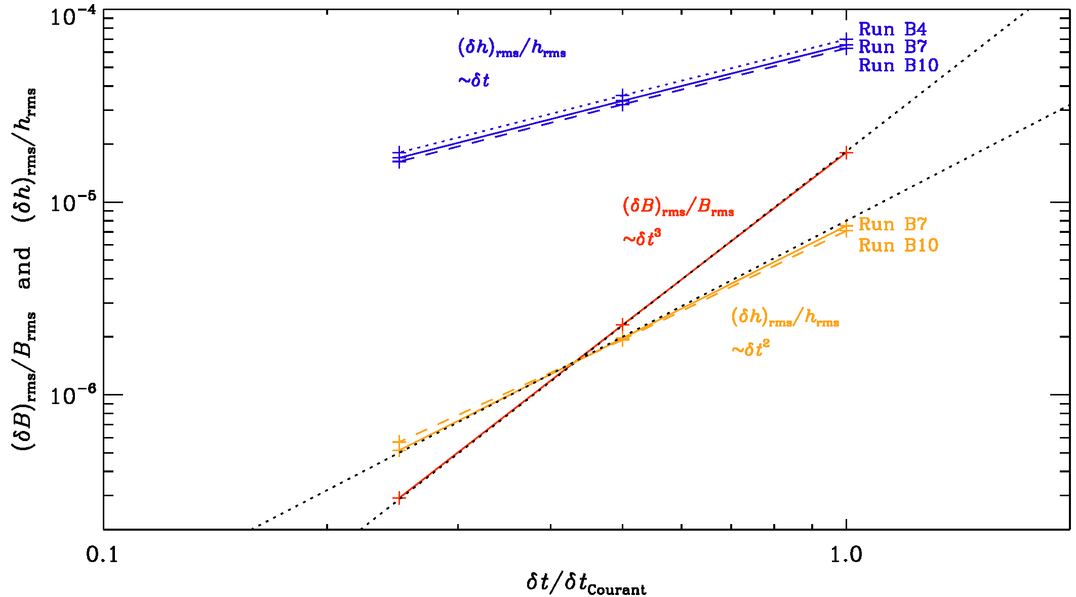
Fig. 2.5 Scalings of the relative error in the magnetic field, \((\delta B)_{\rm rms}/B_{\rm rms}\), and the gravitational strain \((\delta h)_{\rm rms}/h_{\rm rms}\) for GWs generated by the chiral magnetic effect, which leads to an exponentially increasing magnetic field. Low-resolution (\(32^3\)) versions of the Runs B4, B7, and B10 of [BHKRS21].

Analogous to kinetic and magnetic energy and helicity spectra, it is convenient to compute the GW energy and polarization spectra integrated over concentric shells of surface \(\int_{4\pi} k^2 d\Omega_\kv\) in \(\kv\) space:

(2.40)\[\Shdot(k) = \int_{4\pi} \left( | \dthT |^2 + | \dthX |^2 \right) k^2 d\Omega_\kv\]

(2.41)\[\Ahdot(k) = \int_{4\pi} 2 \, \Imag \left( \dthT \dthX^* \right) k^2 d\Omega_\kv\]

The spectra are normalized such that \(\int_0^\infty \Shdot(k) \, dk = \langle \dhT^2 \rangle + \langle \dhX^2 \rangle\) is proportional to the energy density, and \(\int_0^\infty \Ahdot(k) \, dk\) is proportional to the polarized energy density. The \(\Ahdot(k)\) spectra are not to be confused with the magnetic vector potential \(\Av(\xv,t)\).

The corresponding GW energy spectra are:

\[\begin{split}\EGW(k) = \frac{c^2}{32 \pi G} \Shdot(k), \\ \HGW(k) = \frac{c^2}{32 \pi G} \Ahdot(k)\end{split}\]

We also define spectra for the metric tensor perturbation:

\[\begin{split}\Sh(k) = \int_{4\pi} \left( | \tilde{h}_+ |^2 + | \tilde{h}_\times |^2 \right) k^2 d\Omega_\kv, \\ \Ah(k) = \int_{4\pi} 2 \, \Imag ( \tilde{h}_+ \tilde{h}_\times^* ) k^2 d\Omega_\kv\end{split}\]

normalized such that \(\int_0^\infty \Sh(k) \, dk = \hrms^2\) is the mean squared metric tensor perturbation.

Assuming the GW source is constant between two time steps gives an accuracy that scales linearly with the time step \(\delta t\), while the magnetic field, related to the magnetic stress, scales cubically with \(\delta t\). Since \(\tilde{T}_{+/\times}\) are stored in the f-array, it is easy to extract for each wavevector the increment of the stress \(\delta \tilde{T}_{+/\times}\) and use it in an improved update of the GW field:

\[\tilde{h}_{+/\times} = ... + \delta \tilde{T}_{+/\times} \left( 1 - \frac{\sin \omega \delta t}{\omega \delta t} \right)\]

\[\dot{\tilde{h}}_{+/\times} = ... + \delta \tilde{T}_{+/\times} \frac{ 1 - \cos \omega \delta t }{\omega^2 \delta t}\]

This more accurate solver is invoked by setting itorder_GW=2, which results in a quadratic scaling of the error of the GW field; see Fig. 2.5.

2.7. Troubleshooting / Frequently Asked Questions

2.7.1. Download and setup

2.7.1.1. Download forbidden

http://de.wikipedia.org/wiki/GitHub

http://en.wikipedia.org/wiki/SourceForge

A: Both Github and SourceForge are banned from countries on the United States Office of Foreign Assets Control sanction list, including Cuba, Iran, Libya, North Korea, Sudan and Syria; see http://de.wikipedia.org/wiki/GitHub and http://en.wikipedia.org/wiki/SourceForge . As a remedy, you might download a tarball from https://pencil-code.org/. See also Section Download the Pencil Code.

2.7.1.2. When sourcing the sourceme.sh/sourceme.csh file or running pc_setupsrc, I get error messages from the shell, like if: Expression Syntax. or set: Variable name must begin with a letter.

A: This sounds like a buggy shell setup, either by yourself or your system administrator — or a shell that is even more idiosyncratic than the ones we have been working with.

To better diagnose the problem, collect the following information before filing a bug report to us:

1. uname -a
   

2. /bin/csh -v
   

3. echo $version
   

4. echo $SHELL
   

5. ps -p $$
   

6. If you have problems while sourcing the sourceme script:

   1. Unset the PENCIL_HOME variable:

      • for csh and similar:

        unsetenv PENCIL_HOME
        

      • for bash and similar:

        unexport PENCIL_HOME; unset PENCIL_HOME
        

   2. Switch your shell in verbose mode:

      • for csh and similar:

        set verbose; set echo
        

      • for bash and similar:

        set -v; set -x
        

      • then source again.

7. If you have problems with pc_setupsrc, run it with csh in verbose mode:

   /bin/csh -v -x $PENCIL_HOME/bin/pc_setupsrc
   

2.7.2. Compilation

2.7.2.1. Error: relocation truncated to fit

If you get errors while compiling and linking that are similar to:

density.f90:(.text+0x5e0): relocation truncated to fit: R_X86_64_PC32
against symbol `cdata_mp_m_' defined in COMMON section in cdata.o
density.f90:(.text+0x644): additional relocation overflows omitted from the
output
make[2]: *** [start.x] Error 1

A: Your setup is probably too large to fit a normal’ memory model. Please choose a `medium’ or `large’ memory model by adding one of these compiler options to your configuration: :command:-mcmodel=medium` or -mcmodel=large. See Sect. Configuring the code to compile and run on your computer for configuration details. Alternatively, if you use pc_build, you may simply add the respective extension:

pc_build -f GNU-GCC_MPI,GNU-GCC_medium

or for the Intel compiler and a large memory model you would use:

pc_build -f Intel_MPI,Intel_large

2.7.2.2. Linker can’t find the syscalls functions:

ld: 0711-317 ERROR: Undefined symbol: .is_nan_c
ld: 0711-317 ERROR: Undefined symbol: .sizeof_real_c
ld: 0711-317 ERROR: Undefined symbol: .system_c
ld: 0711-317 ERROR: Undefined symbol: .get_env_var_c
ld: 0711-317 ERROR: Undefined symbol: .get_pid_c
ld: 0711-317 ERROR: Undefined symbol: .file_size_c

A: The Pencil Code needs a working combination of a Fortran- and a C-compiler. If this is not correctly set up, usually the linker won’t find the functions inside the syscalls module. If that happens, either the combination of C- and Fortran-compiler is inappropriate (e.g., ifort needs icc), or the compiler needs additional flags, like g95 might need the option -fno-second-underscore and xlf might need the option -qextname. Please refer to Sect. Experimenting with compiler flags, Table Compiler flags for common compilers.

2.7.2.3. Make gives the following error now:

PGF90-S-0017-Unable to open include file: chemistry.h (nochemistry.f90: 43)
  0 inform,   0 warnings,   1 severes, 0 fatal for chemistry

Line 43 of the nochemistry routine, only has 'contains'.

A: This is because somebody added a new module (together with a corresponding nomodule.f90 and a module.h file (chemistry in this case). These files didn’t exist before, so you need to say:

pc_setupsrc

If this does not help, say first make clean and then pc_setupsrc.

2.7.2.4. How do I compile the Pencil Code with the Intel (ifc) compiler under Linux?

A: The Pencil Code should compile successfully with ifc``~6.x, ``ifc``~7.0, sufficiently recent versions of ``ifc 7.1 (you should get the latest version; if yours is too old, you will typically get an internal compiler error’ during compilation of ``src/hydro.f90`), as well as with recent versions of ifort 8.1 (8.0 may also work).

You can find the ifort compiler at <ftp://download.intel.com/software/products/compilers/downloads>_.

On many current (as of November 2003) Linux systems, there is a mismatch between the glibc versions used by the compiler and the linker. To work around this, use the following flag for compiling

FC=ifc -i_dynamic

and set the environment variable

LD_ASSUME_KERNEL=2.4.1; export LD_ASSUME_KERNEL

or

setenv LD_ASSUME_KERNEL 2.4.1

This has solved the problems e.g., on a system with glibc-2.3.2 and kernel 2.4.22.

Thanks to Leonardo J. Milano (http://udel.edu/~lmilano/) for part of this info.

2.7.2.5. I keep getting segmentation faults with start.x when compiling with ifort 8.

A: There was/is a number of issues with ifort 8.0. Make sure you have the latest patches applied to the compiler. A number of things to consider or try are:

1. Compile with the the -static -nothreads flags.

2. Set your stacksize to a large value (but a far too large value may be problematic, too), e.g.

limit stacksize 256m
ulimit -s 256000

3. Set the environment variable KMP_STACKSIZE to a large value (like 100M)

See also http://softwareforums.intel.com/ids/board/message?board.id=11&message.id=1375

2.7.2.6. When compiling with MPI on a Linux system, the linker complains:

mpicomm.o: In function `mpicomm_mpicomm_init_':
mpicomm.o(.text+0x36): undefined reference to `mpi_init_'
mpicomm.o(.text+0x55): undefined reference to `mpi_comm_size_'
mpicomm.o(.text+0x6f): undefined reference to `mpi_comm_rank_'
[...]

A: This is the infamous underscore problem. Your MPI libraries have been compiled with G77 without the option -fno-second-underscore, which makes the MPI symbol names incompatible with other Fortran compilers.

As a workaround, use

MPICOMM = mpicomm_

in Makefile.local. Or, even better, you can set this globally (for the given computer) by inserting that line into the file ~/.adapt-mkfile.inc (see perldoc adapt-mkfile for more details).

2.7.2.7. Compilation stops with the cryptic error message:

f95  -O3 -u -c .f90.f90
Error : Could not open sourcefile .f90.f90
compilation aborted for .f90.f90 (code 1)
make[1]: *** [.f90.o] Error 1

What is the problem?

A: There are two possibilities:

1. One of the variables for make has not been set, so make expands it to the empty string. Most probably you forgot to specify a module in src/Makefile.local. One possibility is that you have upgraded from an older version of the code that did not have some of the modules the new version has.

   Compare your src/Makefile.local to one of the examples that work.

2. One of the variables for make has a space appended to it, e.g., if you use the line

MPICOMM = mpicomm_

• see When compiling with MPI on a Linux system, the linker complains:. With a trailing blank, you will encounter this error message.

• Remove the blank.

• This problem can also occur if you added a new module (and have an empty space after the module name in src/Makefile.src, i.e. CHIRAL=nochiral `), in which case the  compiler will talk about ``circular dependence` for the file nochiral.

2.7.2.8. The code doesn’t compile,

there is a problem with mvar:

make start.x run.x
f95 -O3 -u   -c cdata.f90
Error: cdata.f90, line 71: Implicit type for MVAR
       detected at MVAR@)
[f95 terminated - errors found by pass 1]
make[1]: *** [cdata.o] Error 2

A: Check and make sure that mkcparam (directory $PENCIL_HOME/bin) is in your path. If this doesn’t help, there may be an empty cparam.inc file in your src/ directory. Remove cparam.inc and try again (Note that cparam.inc is automatically generated from the Makefile).

2.7.2.9. Some samples don’t even compile,

As you can see on the web, http://www.nordita.org/software/pencil-code/tests.html.

samples/helical-MHDturb:
    Compiling..           not ok:
  make start.x run.x read_videofiles.x
make[1]: Entering directory `/home/dobler/f90/pencil-code/samples/helical-MHDturb/src'
/usr/lib/lam/bin/mpif95  -O3   -c initcond.f90
/usr/lib/lam/bin/mpif95  -O3   -c density.f90
      use Gravity, only: gravz, nu_epicycle
                                ^
Error 208 at (467:density.f90) : No such entity in the module
Error 355 : In procedure INIT_LNRHO variable NU_EPICYCLE has not been given a type
Error 355 : In procedure POLYTROPIC_LNRHO_DISC variable NU_EPICYCLE has not been given a type
3 Errors
compilation aborted for density.f90 (code 1)
make[1]: *** [density.o] Error 1
make[1]: Leaving directory `/home/dobler/f90/pencil-code/samples/helical-MHDturb/src'
make: *** [code] Error 2

A: Somebody may have checked in something without having run auto-test beforehand. The problem here is that something has been added in one module, but not in the corresponding no-module. You can of course check with svn who it was…

2.7.2.10. Internal compiler error with Compaq/Dec F90

The Dec Fortran optimizer has occasional problems with nompicomm.f90:

make start.x run.x read_videofiles.x
f90  -fast -O3 -tune ev6 -arch ev6  -c cparam.f90
[...]
f90  -fast -O3 -tune ev6 -arch ev6  -c nompicomm.f90
otal vm  2755568      otal vm  2765296        otal vm  2775024
otal vm  2784752      otal...
Assertion failure:  Compiler internal error - please submit problem r...
  GEM ASSERTION, Compiler internal error - please submit problem report
Fatal error in: /usr/lib/cmplrs/fort90_540/decfort90 Terminated
*** Exit 3
Stop.
*** Exit 1
Stop.

A: The occurrence of this problem depends upon the grid size; and the problem never seems to occur with mpicomm.f90, except when ncpus=1. The problem can be avoided by switching off the loop transformation optimization (part of the -O3 optimization), via:

#OPTFLAGS=-fast -O3 -notransform_loops

This is currently the default compiler setting in Makefile, although it has a measurable performance impact (some 8% slowdown).

2.7.2.11. Assertion failure under SunOS

Under SunOS, I get an error message like

user@sun> f90 -c param_io.f90
Assertion failed: at_handle_table[at_idx].tag == VAR_TAG,
                  file ../srcfw/FWcvrt.c, line 4018
f90: Fatal error in f90comp: Abort

A: This is a compiler bug that we find at least with Sun’s WorkShop Compiler version 5.0 00/05/17 FORTRAN 90 2.0 Patch 107356-05. Upgrade the compiler version (and possibly also the operating system): we find that the code compiles and works with version Sun WorkShop 6 update 2 Fortran 95 6.2 Patch 111690-05 2002/01/17 under SunOS version 5.8 Generic_108528-11.

2.7.2.12. After some dirty tricks I got pencil code to compile with MPI, …

> Before that i installed lam-7.1.4 from source.

Goodness gracious me, you shouldn't have to compile your own MPI library.

A: Then don’t use the old LAM-MPI. It is long superseded by open-mpi now. Open-mpi doesn’t need a daemon to be running. I am using the version that ships with Ubuntu (e.g., 9.04):

frenesi:~> aptitude -w 210 search openmpi | grep '^i'

i   libopenmpi-dev - high performance message passing library -- header files
i A libopenmpi1    - high performance message passing library -- shared library
i   openmpi-bin    - high performance message passing library -- binaries
i A openmpi-common - high performance message passing library -- common files
i   openmpi-doc    - high performance message passing library -- man pages

Install that and keep your configuration (Makefile.src and getconf.csh) close to that for frenesi or norlx50. That should work.

2.7.2.13. Error: Symbol ‘mpi_comm_world’ at (1) has no IMPLICIT type

I installed the pencil code on Ubuntu system and tested "run.csh"
in ...\samples\conv-slab.  Here the code worked pretty well.
Nevertheless, running (auto-test), I found there are some errors.
The messages are,
Error: Symbol 'mpi_comm_world' at (1) has no IMPLICIT type
Fatal Error: Error count reached limit of 25.
make[2]: *** [mpicomm_double.o] Error 1
make[2]: Leaving directory
`/home/pkiwan/Desktop/pencil-code/samples/2d-tests/selfgravitating-shearwave/src'
make[1]: *** [code] Error 2
make[1]: Leaving directory
`/home/pkiwan/Desktop/pencil-code/samples/2d-tests/selfgravitating-shearwave/src'
make: *** [default] Error 2
Finally, ### auto-test failed ###

Will it be OK? Or, how can I fix this?

A: Thanks for letting me know about the status, and congratulations on your progress! Those tests that fail are those that use MPI. If your machine is a dual or multi core machine, you could run faster by running under MPI. But this is probably not crucial for you at this point. (I just noticed that there is a ToDo listed in the auto-test command to implement the option not to run the MPI tests, but this hasn’t been done yet. So I guess you can start with the science next.

2.7.2.14. Error: Can’t open included file ‘mpif.h’

It always worked, but now, after some systems upgrade, I get

gfortran -O3 -o mpicomm.o -c mpicomm.f90

Error: Can't open included file 'mpif.h'

When I say locate mpif.h I only get things like

/scratch/ntest/1.2.7p1-intel/include/mpif.h

But since I use FC=mpif90 I thought I don’t need to worry.

A: Since you use FC=mpif90 there must definitely be something wrong with their setup. Try mpif90 -showme or mpif90 -show; the -I` option should say where it looks for ‘mpif.h’. If those directories don’t exist, it’s no wonder that it doesn’t work, and it is time to complain.

2.7.2.15. Compilation fails on MacOS Sonoma or Monterey

I am getting an error which hasn’t been resolved yet. It has something to do with my Mac setup and no one has been able to figure out how to fix it. Maybe you’ve seen this before (at the pc_build stage):

'make -j FFLAGS_DOUBLE=-fdefault-real-8 -fdefault-double-8
CFLAGS_DOUBLE=-DDOUBLE_PRECISION LD_MPI= CFLAGS_FFTW3= FFLAGS_FFTW3=
LD_FFTW3= CFLAGS_FFTW2= FFLAGS_FFTW2= LD_FFTW2= FC=gfortran F77=$(FC)
FFLAGS=-O LDFLAGS_HELPER=-dynamic OMPFFLAGS=-fopenmp OMPLFLAGS=-lgomp
PPFLAGS=-cpp FSTD_95=-std=f95 FSTD_2003=-std=f2003 CC=gcc
CFLAGS=-DFUNDERSC=1 default_to_be' failed: <Inappropriate ioctl for device>

A: You have to use gcc-14. Default (plain gcc) does not work; it is wrongly set up.

2.7.2.16. Compilation fails on Tanmay’s MacOS

In my case the gcc compiler was renamed gcc-14. Once this was fixed, all was good. Could it be that when Mac updates its OS it changes the name of the compiler? I don’t know the backend of the Mac so well.

2.7.2.17. Missing ld_classic on MacOS

While running pc_build, I get an error message saying that -ld_classic is not found.

A: Note that ld_classic is not specifying a library called libd_classic, but is rather an option passed to Apple’s ld binary. type ld should say /usr/bin/ld. This error has been noticed on systems where people tried to install gfortran using anaconda, which pulls in a wrongly configured ld binary. Run conda remove ld64 and use another method, like homebrew, to install gfortran.

2.7.2.18. Further MacOS tips

For further MacOS tips, see also the “Instructions for MacOS installation” on http://pencil-code.nordita.org/doc.php.

2.7.3. Pencil check

2.7.3.1. The pencil check complains for no reason.

A: The pencil check only complains for a reason.

2.7.3.2. The pencil check reports MISSING PENCILS and quits

A: This could point to a serious problem in the code. Check where the missing pencil is used in the code. Request the right pencils, likely based on input parameters, by adapting one or more of the pencil_criteria_MODULE subroutines.

2.7.3.3. The pencil check reports unnecessary pencils

The pencil check reports possible overcalculation... pencil rho (  43) is requested, but does not appear to be required!

A: Such warnings show that your simulation is possibly running too slowly because it is calculating pencils that are not actually needed. Check in the code where the unnecessary pencils are used and adapt one or more of the pencil_criteria_MODULE subroutines to request pencils only when they are actually needed.

2.7.3.4. The pencil check reports that most or all pencils are missing

A: This is typically a thing that can happen when testing new code development for the first time. It is usually an indication that the reference df changes every time you call pde. Check whether any newly implemented subroutines or functionality has a “memory”, i.e. if calling the subroutine twice with the same f gives different output df.

2.7.3.5. Running the pencil check triggers mathematical errors in the code

A: The pencil check puts random numbers in f before checking the dependence of df on the chosen set of pencils. Sometimes these random numbers are inconsistent with the physics and cause errors. In that case you can set lrandom_f_pencil_check=F in &run_pars in run.in. The initial condition may contain many idealized states (zeros or ones) which then do not trigger pencil check errors when lrandom_f_pencil_check=F, even if pencils are missing. But it does prevent mathematical inconsistencies.

2.7.3.6. The pencil check still complains

A: Then you need to look into the how the code and the pencil check operate. Reduce the problem in size and dimensions to find the smallest problem that makes the pencil check fail (e.g., 1x1x8 grid points). At the line of pencil_check.f90 when a difference is found between df_ref and df, add some debug lines telling you which variable is inconsistent and in what place. Often you will be surprised that the pencil check has correctly found a problem in the simulation.

2.7.3.7. The pencil check is annoying so I turned it off

A: Then you are taking a major risk. If one or more pencils are not calculated properly, then the results will be wrong.

2.7.4. Running

2.7.4.1. Why does start.x / start.csh write data with periodic boundary conditions?

A: Because you are setting the boundary conditions in run.in, not in start.in; see Sect. Where to specify boundary conditions. There is nothing wrong with the initial data — the ghost-zone values will be re-calculated during the very first time step.

2.7.4.2. csh problem?

Q: On some rare occasions we have problems with csh not being supported on other machines. (We hope to fix this by contacting the responsible person, but may not be that trivial today!) Oliver says this is a well known bug of some years ago, etc. But maybe in the long run it would be good to avoid csh.

A: These occasions will become increasingly frequent, and eventually for some architectures, there may not even be a csh variant that can be installed.

We never pushed people to use pc_run and friends (and to report corresponding bugs and get them fixed), but if we don’t spend a bit of effort (or annoy users) now, we create a future emergency, where someone needs to run on some machine, but there is no csh and he or she just gets stuck.

We don’t have that many csh files, and for years now it should be possible to compile run without csh (using bin/pc_run) — except that people still fall back on the old way of doing things. This is both cause and consequence of the new way not being tested that much, at least for the corner cases like RERUN, NEWDIR, SCRATCH_DIR.

2.7.4.3. run.csh doesn’t work:

Invalid character ''' in NAMELIST input
Program terminated by fatal I/O error
Abort

A: The string array for the boundary condition, e.g., bcx or bcz is too long. Make sure it has exactly as many elements as nvar is big.

2.7.4.4. Code crashes after restarting

>  > removing mu_r from the namelist just `like that' makes the code
>  > backwards incompatible.
>
>  That means that we can never get rid of a parameter in start.in once we
> have introduced it, right?

A: In the current implementation, without a corresponding cleaning procedure, unfortunately yes.

Of course, this does not affect users’ private changes outside the central svn tree.

2.7.4.5. auto-test gone mad…?

Q: Have you ever seen this before:

giga01:/home/pg/n7026413/cvs-src/pencil-code/samples/conv-slab> auto-test
.

/home/pg/n7026413/cvs-src/pencil-code/samples/conv-slab:
    Compiling..           ok
        No data directory; generating data -> /var/tmp/pencil-tmp-25318
    Starting..            ok
    Running..             ok
    Validating results..Malformed UTF-8 character (unexpected continuation
byte 0x80, with no preceding start byte) in split at
/home/pg/n7026413/cvs-src/pencil-code/bin/auto-test line 263.
Malformed UTF-8 character (unexpected continuation byte 0x80, with no
preceding start byte) in split at
/home/pg/n7026413/cvs-src/pencil-code/bin/auto-test line 263.

A: You are running on a RedHat 8 or 9 system, right?

Set LANG=POSIX in your shell’s startup script and life will be much better.

2.7.4.6. Can I restart with a different number of cpus?

Q: I am running a simulation of nonhelical turbulence on the cluster using MPI. Suppose if I am running a \(128^3\) simulation on 32 cpus/cores i.e.

integer, parameter :: ncpus=32,nprocy=2,nprocz=ncpus/nprocy,nprocx=1
integer, parameter :: nxgrid=128,nygrid=nxgrid,nzgrid=nxgrid

And I stop the run after a bit. Is there a way to resume this run with different number of cpus like this :

integer, parameter :: ncpus=16,nprocy=2,nprocz=ncpus/nprocy,nprocx=1
integer, parameter :: nxgrid=128,nygrid=nxgrid,nzgrid=nxgrid

I understand it has to be so in a new directory but making sure that the run starts from where I left it off in the previous directory.

A: The answer is no, if you use the standard distributed io. There is also parallel io, but I never used it. That would write the data in a single file, and then you could use the data for restart in another processor layout.

2.7.4.7. Can I restart with a different number of cpus?

Q: Is it right that once the simulation is resumed, pencil-code takes the last data from var.dat (which is the current snapshot of the fields)? If that is true, then, is it not possible to give that as the initial condition for the run in the second directory (with changed "ncpus")? Is there a mechanism already in place for that?

A: Yes, the code restarts from the last var.dat. It is written after a successful completion of the run, but it crashes or you hit a time-out, there will be a var.dat that is overwritten every isave timesteps. If the system stops during writing, some var.dat files may be corrupt or have the wrong time. In that case you could restart from a good VAR file, if you have one, using, e.g.,

restart-new-dir-VAR . 46

where 46 is the number of your VAR file, i.e., VAR46 im this case. To restart in another directory, you say, from the old run directory,

restart-new-dir ../another_directory

Hope this helps. Look into pencil-code/bin/restart-new-dir to see what it is doing.

2.7.4.8. fft_xyz_parallel_3D: nygrid needs to be an integer multiple…

Q: I just got an:

fft_xyz_parallel_3D: nygrid needs to be an integer multiple of nprocy*nprocz

In my case, nygrid=2048, nprocy=32, and nprocz=128, so nprocy*nprocz=4096. In other words, 2048 needs to be a multiple of 4096. But isn’t this the case then?

A: No, because 2048 = 0.5 * 4096 and 0.5 is not an integer. Maybe try either setting nprocz=64 or nprocy=64. You could compensate the change of ncpus with the \(x\)-direction. For \(2048^3\) simulations, nprocy=32 and nprocz=64 would be good. A list of good meshes is given in Table 2.4.

2.7.4.9. Unit-agnostic calculations?

Q: The manual speaks about unit-agnostic calculations, stating that one may choose to interpret the results in any (consistent) units, depending on the problem that is solved at hand. So, for example, if I chose to run the 2d-tests/battery_term simulation for an arbitrary number of time-steps and then choose to examine the diagnostics, am I correct in assuming the following:

1) [Brms] = Gauss (as output by unit_magnetic, before the run begins)
2) [t] = s (since the default unit system is left as CGS)
3) [urms] = cm/s (again, as output by unit_velocity, before the run begins)
4) and etc. for the units of the other diagnostics

A: Detailed correspondence on this item can be found on: <https://groups.google.com/forum/?fromgroups#!topic/pencil-code-discuss/zek-uYNbgXI>_ There is also working material on unit systems under <http://www.nordita.org/~brandenb/teach/PencilCode/MixedTopics.html>_ with a link to <http://www.nordita.org/~brandenb/teach/PencilCode/material/AlfvenWave_SIunits/>_ Below is a pedagogical response from Wlad Lyra:

In the sample battery-term, the sound speed cs0=1 sets the unit of
velocity. Together with the unit of length, that sets your unit of
time. The unit of magnetic field follows from the unit of velocity,
density, and your choice of magnetic permittivity, according to the
definition of the Alfven velocity.

If you are assuming cgs, you are saying that your sound speed cs0=1
actually means [U]=1 cm/s. Your unit of length is equivalently 1 cm,
and therefore the unit of time is [t] = [L]/[U]=1 s. The unit of
density is [rho] = 1 g/cm^3. Since in cgs vA=B/sqrt(4*pi * rho), your
unit of magnetic field is [B] = [U] * sqrt([rho] * 4*pi) ~= 3.5
sqrt(g/cm) / s = 3.5 Gauss.

If instead you are assuming SI, you have cs0=1 assuming that means
[U]=1 m/s and rho0=1 assuming that to mean [rho]=1 kg/m^3. Using [L]=1
m, you have still [t]=1 s, but now what appears as B=1 in your output
is actually [B] = [U] * sqrt (mu * [rho]) = 1 m/s * sqrt(4*pi * 1e-7
N*A-2  1 kg/m^3)  ~= 0.0011210 kg/(s^2*A) ~ 11 Gauss.

You can make it more interesting and use units relevant to the
problem. Say you are at the photosphere of the Sun. You may want to
use dimensionless cs0=1 meaning a sound speed of 10 km/s.  Your
appropriate length can be a megameter. Now your time unit is
[t]=[L]/[U] = 1e3 km/ 10 km/s = 10^2 s, i.e., roughly 1.5 minute. For
density, assume rho=2x10-4 kg/m^3, typical of the solar photosphere.
Your unit of magnetic field is therefore [B] = [U] * sqrt([rho] *
4*pi) = 1e6 cm/s * sqrt(4*pi * 2e-7 g/cm^3) ~ 1585.33 Gauss.

Notice that for mu0=1 and rho0=1 you simply have vA=B. Then you can
conveniently set the field strength by your choice of plasma beta (=
2*cs^2/vA^2). There's a reason why we like dimensionless quantities!

2.7.5. Visualization FAQ

2.7.5.1. start.pro doesn’t work:

Reading grid.dat..
Reading param.nml..
% Expression must be a structure in this context: PAR.
% Execution halted at:  $MAIN$            104
/home/brandenb/pencil-code/runs/forced/hel1/../../../idl/start.pro

A: You don’t have the subdirectory data/ in your IDL variable !path. Make sure you source sourceme.csh/sourceme.sh or set a sufficient IDL path otherwise.

2.7.5.2. start.pro doesn’t work (2):

Isn’t there some clever (or even trivial) way that one can avoid the annoying error messages that one gets, when running e.g., .r rall after a new variable has been introduced in “idl/varcontent.pro”? Ever so often there’s a new variable that can’t be found in my param2.nml – this time it was IECR, IGG, and ILNTT that I had to circumvent…

A: The simplest solution is to invoke NOERASE, i.e. say

touch NOERASE
start.csh

or, alternatively, start_run.csh. What it does is that it reruns src/start.x with a new version of the code; this then produces all the necessary auxiliary files, but it doesn’t overwrite or erase the var.dat and other VAR and slice files.

2.7.5.3. Something about tag name undefined:

Q: In one of my older run directories I can’t read the data with idl anymore. What should I do? It says something like

Reading param.nml..
% Tag name LEQUIDIST is undefined for structure <Anonymous>.
% Execution halted at: $MAIN$            182
  /people/disk2/brandenb/pencil-code/idl/start.pro

A: Go into data/param.nml and add , LEQUIDIST=T anywhere in the file (but before the last slash).

2.7.5.4. Something INC in start.pro

Q: start doesn’t even work:

% Compiled module: $MAIN$.
nname=      11
Reading grid.dat..
Reading param.nml..
Can't locate Namelist.pm in INC (INC contains: /etc/perl /usr/local/lib/perl/5.8.4 /usr/local/share/perl/5.8.4 /usr/lib/perl5 /usr/share/perl5 /usr/lib/perl/5.8 /usr/share/perl/5.8 /usr/local/lib/site_perl .) at /home/brandenb/pencil-code/bin/nl2idl line 49.
BEGIN failed--compilation aborted at /home/brandenb/pencil-code/bin/nl2idl line 49.

A: Go into $PENCIL_HOME and say svn up sourceme.csh and/or svn up sourceme.sh. (They were just out of date.)

2.7.5.5. nl2idl problem when reading param2.nml

Q: Does anybody encounter a backward problem with nl2idl? The file param*.nml files are checked in under pencil-code/axel/couette/SStrat128a_mu0.20_g2 and the problem is below.

 at /people/disk2/brandenb/pencil-code/bin/nl2idl line 120
HCOND0= 0.0,HCOND1= 1.000000,HCOND2= 1.000000,WIDTHSS= 1.192093E-06,MPOLY0=
^------  HERE
 at /people/disk2/brandenb/pencil-code/bin/nl2idl line 120

A: The problem is the ifc compiler writing the following into the namelist file:

COOLING_PROFILE='gaussian                 ',COOLTYPE='Temp
'COOL= 0.0,CS2COOL= 0.0,RCOOL= 1.000000,WCOOL= 0.1000000,FBOT= 0.0,CHI_T= 0.0

If you add a comma after the closing quote:

COOLING_PROFILE='gaussian                 ',COOLTYPE='Temp
',COOL= 0.0,CS2COOL= 0.0,RCOOL= 1.000000,WCOOL= 0.1000000,FBOT= 0.0,CHI_T= 0.0

things will work.

Note that ifc cannot even itself read what it is writing here, so if this happened to occur in param.nml, the code would require manual intervention after each start.csh.

2.7.5.6. Spurious dots in the time series file

Q: Wolfgang, you explained it to me once, but I forget. How can one remove spurious dots after the timestep number if the time format overflows?

A: I don’t know whether it exists anywhere, but it’s easy. In Perl you’d say

perl -pe 's/^(\s*[-0-9]+)\.([-0-9eEdD])/$1 $2/g'

and in sed (but that’s harder to read)

sed 's/^\( *[-0-9]\+\)\.\([-0-9eEdD]\)/\1 \2/g'

2.7.5.7. Problems with pc_varcontent.pro

Q:

% Subscript range values of the form low:high must be >= 0, < size, with low
<= high: VARCONTENT.
% Error occurred at: PC_VARCONTENT     391
  /home/brandenb/pencil-code/idl/read/pc_varcontent.pro
%                    PC_READ_VAR       318
  /home/brandenb/pencil-code/idl/read/pc_read_var.pro
%                    $MAIN$

A: Make sure you don’t have any unused items in your src/cparam.local such as

! MAUX CONTRIBUTION 3
! COMMUNICATED AUXILIARIES 3

They would leave gaps in the counting of entries in your data/index.pro file.

2.7.6. Programming new slices

Q: I’m creating a new special module with a few new variables f(:,:,:,inew1), f(:,:,:,inew2) etc. I’m wondering how to add new output of slices (i.e. video files) of these new variables (say p%inew1) and their combinations (say p%inew1**2+p%inew2**2)? I tried to look into other modules to find an example but got confused. If someone could clarify the calling tree it would be great!

A: Best you look into hydro.f90. For slices, which contain simply f-array variables, you do something like

case ('uu'); call assign_slices_vec(slices,f,iuu)

in get_slices_hydro. For slices, which contain derived quantities like your p%inew1**2+p%inew2**2, you have to declare slice buffers as for divu in hydro (divu_xy etc.), you have to allocate them like

if (ivid_divu/=0) call alloc_slice_buffers(divu_xy,divu_xz, &
  divu_yz,divu_xy2,divu_xy3,divu_xy4,divu_xz2,divu_r)

to fill them in calc_diagnostics_special like

if (ivid_divu/=0) call store_slices(p%divu,divu_xy,divu_xz, &
  divu_yz,divu_xy2,divu_xy3,divu_xy4,divu_xz2,divu_r)

and finally to store them in get_slices_special like

call assign_slices_scal(slices,divu_xy,divu_xz,divu_yz, &
  divu_xy2,divu_xy3,divu_xy4,divu_xz2,divu_r)

2.7.7. General questions

2.7.7.1. Installation procedure

2.7.7.1.1. Why don’t you use GNU autoconf/automake for installation of the PENCIL CODE?

A: What do you mean by “installation”? Unlike the applications that normally use autoconf, the :Pencil Code: is neither a binary executable, nor a library that you compile once and then dump somewhere in the system tree. Autoconf is the right tool for these applications, but not for numerical codes, where the typical compilation and usage pattern is very different:

You have different directories with different Makefile.local settings, recompile after introducing that shiny new term in your equations, etc. Moreover, you want to sometimes switch to a different compiler (but just for that run directory) or another MPI implementation. Our adapt-mkfile approach gives you this flexibility in a reasonably convenient way, while doing the same thing with autoconf would be using that system against most of its design principles.

Besides, it would really get on my (WD’s) nerves if I had to wait two minutes for autoconf to finish before I can start compiling (or maybe 5–10 minutes if I worked on a NEC machine…).

Finally, if you have ever tried to figure out what a configure script does, you will appreciate a comprehensible configuration system.

2.7.7.2. Small numbers in the code

What is actually the difference between epsi, tini and tiny?

A:

F90 has two functions epsilon() and tiny(), with

  epsilon(x) = 1.1920929e-07
  tiny(x)    = 1.1754944e-38
(and then there is huge(x) = 3.4028235e+38)
for a single-precision number x.

epsilon(x) is the smallest number that satisfies
  1+epsilon(1.) /= 1 ,
while tiny(x) is the smallest number that can be represented without
precision loss.

In the code we have variants hereof,
   epsi=5*epsilon(1.0)
   tini=5*tiny(1.0)
   huge1=0.2*huge(1.0)
that have added safety margins, so we don't have to think about doing
things like 1/tini.

So in sub.f90,
  -      evr = evr / spread(r_mn+epsi,2,3)
did (minimally) affect the result for r_mn=O(1), while the correct version
  +      evr = evr / spread(r_mn+tini,2,3)
only avoids overflow.

2.7.7.3. Why do we need a /lphysics/ namelist in the first place?

Wolfgang answered on 29 July 2010: “cdata.f90 has the explanation”

! Constant 'parameters' cannot occur in namelists, so in order to get the
! now constant module logicals into the lphysics name list...
! We have some proxies that are used to initialize private local variables
! called lhydro etc, in the lphysics namelist!

So the situation is this: we want to write parameters like ldensity to param.nml so IDL (and potentially octave, python, etc.) can know whether density was on or not. To avoid confusion, we want them to have exactly their original names. But we cannot assemble the original ldensity etc. constants in a namelist, so we have to define a local ldensity variable. And to provide it with the value of the original cdata.ldensity, we need to transfer the value via ldensity_var. That’s pretty scary, although it seems to work fine. I can track the code back to the big eos_merger commit, so it may originate from that branch. One obvious problem is that you have to add code in a number of places (the ldensity -> ldensity_var assignment and the local definition of ldensity) to really get what you need. And when adding a new boolean of that sort to cdata.f90, you may not even have a clue that you need all the other voodoo.

2.7.7.4. Can I run the code on a Mac?

A: Macs work well for Linux stuff, except that the file structure is slightly different. Problems when following Linux installs can usually be traced to the PATH. For general reference, if you need to set an environment variable for an entire OS-X login session, google environment.plist. That won’t be needed here.

For a Mac install, the following should work:

1. Install Dev Tools (an optional install on the MacOS install disks). Unfortunately, last time I checked the svn version that comes with DevTools is obsolete. So:

2. Install MacPorts (download from web). Note that MacPorts installs to a non-standard location, and will need to be sourced. The installation normally drops an appropriate line in .profile. If it does so, make sure that line gets sourced. Otherwise

export PATH=/opt/local/bin:/opt/local/sbin:$PATH
export MANPATH=/opt/local/share/man:$MANPATH

3. Install g95 (download from web). Make sure it is linked in /bin.

4. execute macports svn install

5. download the pencil-code and enjoy.

Note

the above way to get svn works. It takes a while however, so there are certainly faster ways out there. If you already have a non-obsolete svn version, use that instead.

2.7.7.5. Wrong user-id in commit emails

Why does it say

From: 'Philippe Bourdin' via pencil-code-commits
      <pencil-code-commits@googlegroups.com>

when the committing author is not Philippe?

A: The associated email addresses in account.pencil-code.org should be the same as what is registered in github as your primary email address.

2.7.7.6. Pencil Code discussion forum

Do I just need to send an email somewhere to subscribe or what?

A: The answer is yes; just go to:

http://groups.google.com/group/pencil-code-discuss

2.7.7.7. The manual

It would be a good idea to add this useful information in the manual, no?

A: When you have added new stuff to the code, don’t forget to mention this in the pencil-code/doc/manual.tex file.

Again, the answer is yes; just go to:

cd pencil-code/doc/
vi manual.tex
svn ci -m "explanations about a new module in the code"

2.8. References

[Abramowitz-Stegun]

Abramowitz, A., & Stegun, I. A. (1984). Pocketbook of Mathematical Functions. Harri Deutsch, Frankfurt.

[BHB11]

Babkovskaia, N., Haugen, N. E. L., & Brandenburg, A. (2011). J. Comp. Phys., 230(1), 12. A high-order public domain code for direct numerical simulations of turbulent combustion. (arXiv:1005.5301)

[BB14]

Barekat, A., & Brandenburg, A. (2014). Astron. Astrophys., 571, A68. “Near-polytropic stellar simulations with a radiative surface.”

[Ref-2]

Brandenburg, A. (2001). Astrophys. J., 550, 824–840. “The inverse cascade and nonlinear alpha-effect in simulations of isotropic helical hydromagnetic turbulence.”

[Ref-1]

Brandenburg, A. (2003). In Advances in non-linear dynamos (A. Ferriz-Mas & M. Núñez Jiménez, Eds.), The Fluid Mechanics of Astrophysics and Geophysics, Vol. 9, pp. 269–344. Taylor & Francis, London and New York. Available at http://arXiv.org/abs/astro-ph/0109497

[Ref-4]

Brandenburg, A., & Dobler, W. (2001). Astron. Astrophys., 369, 329–338. “Large scale dynamos with helicity loss through boundaries.”

[BH01]

Brandenburg, A., & Hazlehurst, J. (2001). Astron. Astrophys., 370, 1092–1102. “Evolution of highly buoyant thermals in a stratified layer.”

[BK17]

Brandenburg, A., & Kahniashvili, T. (2017). Phys. Rev. Lett., 118, 055102. “Classes of hydrodynamic and magnetohydrodynamic turbulent decay.”

[BHKRS21]

Brandenburg, A., He, Y., Kahniashvili, T., Rheinhardt, M., & Schober, J. (2021). Astrophys. J., 911, 110. “Gravitational waves from the chiral magnetic effect.”

[BS02]

Brandenburg, A., & Sarson, G. R. (2002). Phys. Rev. Lett., 88, 055003. “The effect of hyperdiffusivity on turbulent dynamos with helicity.”

[BDS02]

Brandenburg, A., Dobler, W., & Subramanian, K. (2002). Astron. Nachr., 323, 99–122. “Magnetic helicity in stellar dynamos: new numerical experiments.”

[BEO96]

Brandenburg, A., Enqvist, K., & Olesen, P. (1996). Phys. Rev. D, 54, 1291–1300. “Large-scale magnetic fields from hydromagnetic turbulence in the very early universe.”

[BJNRST96]

Brandenburg, A., Jennings, R. L., Nordlund, Å., Rieutord, M., Stein, R. F., & Tuominen, I. (1996). J. Fluid Mech., 306, 325–352. “Magnetic structures in a dynamo simulation.”

[BKMRPTV17]

Brandenburg, A., Kahniashvili, T., Mandal, S., Roper Pol, A., Tevzadze, A. G., & Vachaspati, T. (2017). Phys. Rev. D, 96, 123528. “Evolution of hydromagnetic turbulence from the electroweak phase transition.”

[BMS95]

Brandenburg, A., Moss, D., & Shukurov, A. (1995). MNRAS, 276, 651–662. “Galactic fountains as magnetic pumps.”

[BNST95]

Brandenburg, A., Nordlund, Å., Stein, R. F., & Torkelsson, U. (1995). Astrophys. J., 446, 741–754. “Dynamo-generated turbulence and large scale magnetic fields in a Keplerian shear flow.”

[Collatz66]

Collatz, L. (1966). The numerical treatment of differential equations. Springer-Verlag, New York, p. 164.

[Dobler06]

Dobler, W., Stix, M., & Brandenburg, A. (2006). Astrophys. J., 638, 336–347. “Convection and magnetic field generation in fully convective spheres.”

[Dur08] (1,2)

Durrer, R. (2008). The Cosmic Microwave Background. Cambridge University Press.

[Gammie2001] (1,2)

Gammie, C. F. (2001). Astrophys. J., 553, 174–183. “Nonlinear outcome of gravitational instability in cooling, gaseous disks.”

[GNG87]

Goodman, J., Narayan, R., & Goldreich, P. (1987). Month. Not. Roy. Soc., 225, 695–711. “The stability of accretion tori — II. Nonlinear evolution to discrete planets.”

[HB04a]

Haugen, N. E. L., & Brandenburg, A. (2004). Phys. Rev. E, 70, 026405. “Inertial range scaling in numerical turbulence with hyperviscosity.”

[HockneyEastwood1981]

Hockney, R. W., & Eastwood, J. W. (1981). Computer Simulation Using Particles. McGraw-Hill, New York.

[HTM84]

Hurlburt, N. E., Toomre, J., & Massaguer, J. M. (1984). Astrophys. J., 282, 557–573. “Two-dimensional compressible convection extending over multiple scale heights.”

[kim87]

Kim, J., Moin, P., & Moser, R. (1987). J. Fluid Mech., 177, 133. “Turbulence statistics in fully developed channel flow at low Reynolds number.”

[KW90]

Kippenhahn, R., & Weigert, A. (1990). Stellar structure and evolution. Springer, Berlin.

[KR80]

Krause, F., & Rädler, K.-H. (1980). Mean-Field Magnetohydrodynamics and Dynamo Theory. Akademie-Verlag, Berlin; also Pergamon Press, Oxford.

[Lele92]

Lele, S. K. (1992). J. Comp. Phys., 103, 16–42. “Compact finite difference schemes with spectral-like resolution.”

[MTW]

Misner, C. W., Thorne, K. S., & Wheeler, J. A. (1973). Gravitation. San Francisco: W. H. Freeman and Co., p. 213.

[MTBM09]

Mitra, D., Tavakol, R., Brandenburg, A., & Moss, D. (2009). Astrophys. J., 697, 923–933. “Turbulent dynamos in spherical shell segments of varying geometrical extent.” (arXiv:0812.3106)

[NG95]

Nordlund, Å., & Galsgaard, K. (1995). A 3D MHD code for Parallel Computers. Available at http://www.astro.ku.dk/~aake/NumericalAstro/papers/kg/mhd.ps.gz

[NS90]

Nordlund, Å., & Stein, R. F. (1990). Comput. Phys. Commun., 59, 119. “3-D simulations of solar and stellar convection and magnetoconvection.”

[Ole97]

Olesen, P. (1997). Phys. Lett. B, 398, 321. “Inverse cascades and primordial magnetic fields.”

[NR]

Press, W., Teukolsky, S., Vetterling, W., & Flannery, B. (1996). Numerical Recipes in Fortran 90 (2nd ed.). Cambridge.

[SH88]

Stanescu, D., & Habashi, W. G. (1988). J. Comp. Phys., 143, 674. “2N-storage low dissipation and dispersion Runge–Kutta schemes for computational acoustics.”

[2Nstorage]

Williamson, J. H. (1980). J. Comp. Phys., 35, 48. “Low-storage Runge–Kutta schemes.”

[JOSS]

Pencil Code Collaboration. (2021). J. Open Source Software, 6, 2807. “The Pencil Code, a modular MPI code for partial differential equations and particles: multipurpose and multiuser-maintained.”

[Porter22]

Porter, T. A., Jóhannesson, G., & Moskalenko, I. V. (2022). Astrophys. J. Supp., 262, 30. “The GALPROP Cosmic-ray Propagation and Nonthermal Emissions Framework: Release v57.”

[mcmodel]

Intel. Fortran Compiler Developer Guide and Reference – mcmodel. https://software.intel.com/en-us/fortran-compiler-developer-guide-and-reference-mcmodel