Ultra quick start guide

Welcome to the Ultra Quick Start Guide — the fastest way to run your first PENCIL CODE simulation without even getting your hands dirty. If the Quick Start Guide was a coffee, this one is an espresso shot. The Full User Manual? That’s your five-course meal with footnotes.

This document is for the impatient, the curious, or anyone who just wants to see PENCIL CODE come to life before lunch.

Required software

All you need is Docker — the container platform that lets you borrow someone else’s perfectly prepared environment so you can skip the compiler setup and get straight to science.

Download the Pencil Code

For the long story, see Download the Pencil Code. The short version: use Git.

git clone https://github.com/pencil-code/pencil-code.git

That will create a directory named pencil-code containing everything you need to run the examples below. You now have the full source at your fingertips — ready to simulate, experiment, or just admire from a safe distance.

Running with Docker

If you want to skip all compilation steps and jump straight into running a simulation, you can use the Docker setup described below. It automatically downloads all necessary packages and configures the latest Pencil Code environment, so you can start experimenting in minutes — no compiler installation required.

This method is perfect if you want to test-drive PENCIL CODE or run a self-contained example without installing a single library on your machine.

It can compile both MPI and non-MPI simulations.

Limitation

Cannot yet be used on supercomputers.

Getting the Docker files

The Docker setup lives in a few simple text files that tell Docker how to build and start the environment.

They are included in the Pencil Code repository under ~/pencil-code/doc/readthedocs/pencil-docker.

If you ever wanted to see how an entire computational environment fits inside a few lines of YAML — this is your chance.

Starting up

Move to the Docker directory and start the container:

cd ~/pencil-code/doc/readthedocs/pencil-docker
run_docker

Tip

The first time you build the container, it may take several minutes as it downloads compilers and all necessary libraries. Once the container is built, subsequent starts will be much faster. (Think of it as caching your future patience.)

You are now inside the container — ready to run, compile, or explore the code as if it were installed locally.

This container mounts the pencil-code directory as a volume and works inside that directory, so any data created within the container will also be available outside it.

Now you can execute any Pencil pc_ command without worrying about compilers and packages.

Stopping the container

If your terminal is attached to the container (following the run_docker command, see above), simply press Ctrl-C. The container will stop and you will return to your terminal session on the host machine.
From any other terminal, run the docker stop command and specify the name of the container:
```
docker stop pencil
```

Running GUI applications

The container is configured to display GUI applications on the host. For a quick test, try:

xclock

If the window does not appear, you may need to grant X11 access on your host before you run the container (if the container is running, you will have to stop it, run the following command, and then restart it):

xhost +

After that, you can use visualization tools such as matplotlib and call plt.show() from inside the container — and the plot windows will appear on your desktop as usual. (No magic, just Docker sorcery.)

Running a test simulation

To verify that everything works correctly, execute the included test script. It compiles and runs the same sample problem used in the Quick start guide example (samples/conv-slab), so the output should be the same as there.

$ execute-test

This script creates a docker-test directory inside pencil-code, copies the example sample, moves there, compiles, and runs the sample problem - producing output similar to the following:

--it-----t-------dt------urms----umax----rhom----ssm----dtc---dtu---dtnu-dtchi-
  0.00 6.793E-03  0.0063  0.0956 14.4708 -0.4460 0.978 0.025 0.207 0.345
  0.07 6.793E-03  0.0056  0.0723 14.4708 -0.4464 0.978 0.019 0.207 0.345
  0.14 6.793E-03  0.0053  0.0471 14.4709 -0.4467 0.978 0.019 0.207 0.345
  0.20 6.793E-03  0.0056  0.0413 14.4708 -0.4471 0.978 0.017 0.207 0.346
  0.27 6.793E-03  0.0058  0.0449 14.4708 -0.4475 0.978 0.013 0.207 0.346

Simulation finished after           41  time-steps

If you see similar output, your Docker setup is fully operational.

Important

Running the script again will overwrite pencil-code/docker-test/conv-slab. Consider it a clean slate for your next experiment.

Post-processing and visualizing data

Once your simulation has finished, you can post-process the results either from within the container or outside it. Since the container shares the pencil-code directory with your host system, all your data are right where you expect them — no hunting through mysterious Docker volumes.

You can use Python, IDL (via GDL), or any other familiar tools. The container already includes everything you need for both.

Testing the Python module

The container also includes the Python interface to the Pencil Code. To verify that it works, start Python inside the container and try importing the module:

$ python3
Python 3.10.12 (main, Aug 15 2025, 14:32:43) [GCC 11.4.0] on linux
>>> import pencil
>>>

If that runs without errors, the Python tools are ready for use — no extra setup, no environment juggling.

In the following, we’ll use the same test simulation (the one you just ran in docker-test/conv-slab) to demonstrate how to explore results using the pencil module.

Using the `pencil` module

Let’s open the time series data created by the test run. (Yes, you’re about to plot something that was born inside a container.)

import pencil as pc
import matplotlib.pyplot as plt

Read the time series generated by the simulation data/time_series.dat

>>> ts = pc.read.ts()
Read 5 lines.

If write ts. and your press tab you will see all the options:

>>> ts.
ts.dt     ts.dtchi  ts.dtu    ts.keys   ts.rhom   ts.t      ts.urms
ts.dtc    ts.dtnu   ts.it     ts.read(  ts.ssm    ts.umax
>>> ts.

To plot the RMS velocity urms, simply do:

plt.plot(ts.t,ts.urms)
plt.xlabel("Time")
plt.ylabel("u_rms")
plt.title("Time evolution of u_rms")
plt.show()

You should get something like:

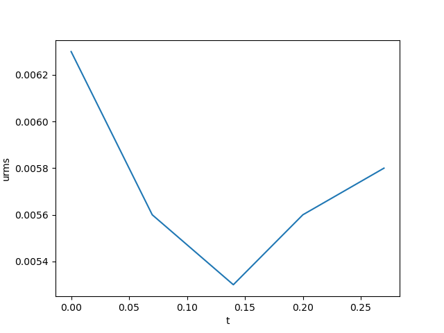
../_images/qguide_convlab_turms.png — Fig. 1 Evolution of the urms in the conv-slab simulation. Python post-processing inside the container.

Some examples of postprocessing with Python can be found in the python tutorials.

Using IDL

Prefer IDL? The container includes GDL, a free and open-source clone of IDL, so you can also run IDL scripts inside the container.

$ idl
GDL> pc_read_ts, obj=ts
GDL> help, ts, /structure
GDL> plot, ts.t, ts.urms,/ynozero

Which produces:

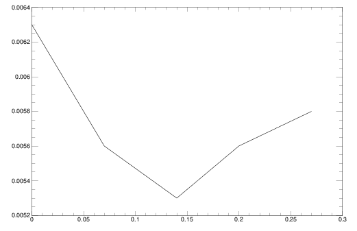
../_images/qguide_convlab_turms_idl.png — Fig. 2 Evolution of the urms in the conv-slab simulation.. IDL post-processing inside the container.

Tip

Feeling energized? Now that you’ve had your digital espresso, you’re ready to dive deeper — from tweaking parameters to exploring the Full Manual, the world of Pencil Code awaits.