Convection simulation: conv-slab

Scientific background

This is one of the first benchmark setups used in the Pencil Code, motivated by the seminal work of Hurlburt & Toomre (1984) on convection in stellar atmospheres. The present implementation is described in Brandenburg et al. (1996).

The simulation models Rayleigh-Bénard convection in a stratified layer, similar to convection dynamics in the solar convection zone. The physical setup consists of:

A vertical layer of fluid with a subadiabatic entropy stratification below (stable layer) and a superadiabatic layer above (unstable layer where convection occurs)
Periodic boundary conditions in the horizontal (x, y) directions
Closed (symmetric/antisymmetric) boundary conditions in the vertical (z) direction
Rotation about the vertical axis (angular velocity Ω = 0.1)
Density stratification that creates buoyancy-driven flows

The convection is driven by the entropy gradient: the superadiabatic layer is unstable and develops strong convective plumes that transport heat upward. The simulation captures how rising hot fluid and sinking cold fluid organize into coherent structures, and how rotation affects this organization through Coriolis forces.

References:: Brandenburg, A., Jennings, R. L., Nordlund, Å., Rieutord, M., Stein, R. F., & Tuominen, I.: 1996, ``Magnetic structures in a dynamo simulation,’’ J. Fluid Mech. 306, 325-352

:pencil-code/samples/conv-slab

Configuration of the simulation

This sample is in the directory:

pencil-code/samples/conv-slab

Configuration files: as in any Pencil Code simulation, the important configuration files are:

src/cparam.local: Setup the number of processors. In this case, two processors divide the domain to handle the computation efficiently.
run.in: Runtime parameters controlling the simulation evolution and physical setup. Includes:
- Time stepping: nt=41, it1=10, isave=200 (41 timesteps, save every 200 steps). Alternative configuration commented: nt=4000 for extended free evolution.
- Boundary conditions: Periodic in x,y directions; symmetric/antisymmetric in z
- Physical parameters:
  - Rotation: Omega=0.1 — Angular velocity about the vertical axis, creating Coriolis forces that organize convective structures
  - Gravity: Constant downward (gravz=-1.)
  - Entropy cooling: wheat=0.1, cool=15., wcool=0.2 — Radiative cooling in the upper layer to maintain superadiabatic stratification
  - Thermal conductivity: K-profile with hcond0=8.e-3 — Heat diffusion process
  - Viscosity: nu=4e-3 — Kinematic viscosity controlling dissipation
- Numerical stability: cdtv=0.30, cdt=0.4 — Courant numbers limiting timestep size
start.in: Initialization parameters that set up the initial stratification and velocity perturbations:
- Domain size: Lxyz = 1., 1., 2. — A rectangular domain with height twice the horizontal extent
- Box position: xyz0 = -0.5, -0.5, -0.68 — Centered horizontally, extends from -0.68 to 1.32 vertically
- Density profile: initlnrho='piecew-poly' — Piecewise polytropic density stratification, smoother than step functions
- Entropy profile: initss='piecew-poly' with mpoly0=1., mpoly1=3., mpoly2=0. — Creates the superadiabatic layer (unstable region where convection initiates)
- Velocity seed: inituu='up-down' with ampluu=1.e-1 — Weak perturbations to trigger convection instability
print.in: Diagnostic variables written to time series file time_series.dat:
- urms — RMS velocity (monitor of convective vigor)
- umax — Maximum velocity
- rhom, ssm — Mean density and entropy
- dt* — Timestep diagnostics (dtc, dtu, dtnu, dtchi)
video.in: Variables saved to video files for visualization:
- uu — Velocity field (shows convective plumes)
- lnrho — Log density (reveals stratification and density perturbations)
xyaver.in: Specifies variables for xy-averaged diagnostics used in energy flux analysis:
- fkin — Kinetic energy flux
- frad — Radiative flux
- fconv — Convective flux
- fcool — Cooling flux
- Other thermodynamic and dynamical quantities for vertical profiles

Typical runtime: For 4000 timesteps with two processors, runtime is ~30-60 seconds on modern hardware.

Note on Configuration: To reproduce the plots and analysis in this tutorial, use the following settings in run.in:

nt=4000, it1=10, isave=10, itorder=3
dsnap=0.2, dvid=0.2

These parameters ensure adequate temporal resolution for capturing the convection dynamics and sufficient data sampling for the flux analysis.

Useful check during run time

While the simulation is running, you can monitor its progress using Python and the Pencil Code analysis tools. Here are several useful diagnostic checks:

Basic diagnostics - Monitoring convective activity:

import pencil as pc
import matplotlib.pyplot as plt

# Create simulation object
sim = pc.sim.simulation(sdir)

# Read time series
ts = pc.read.ts(sim=sim)

# Create figure

fig, ax = plt.subplots(figsize=(10, 8),constrained_layout = True)

# Monitor RMS velocity (main indicator of convective vigor)


ax.plot(ts.t,ts.urms)

ax.set_xlabel('Time')
ax.set_ylabel('RMS velocity')
ax.set_title('Convection Intensity Evolution')
ax.grid()
plt.show()

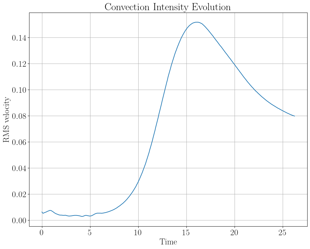
You can download the python script inside the corresponding python folder: conv-slab/python/ptvsurms.py

Tracking maximum velocity and mean quantities:

# Create simulation object
sim = pc.sim.simulation(sdir)

# Read time series
ts = pc.read.ts(sim=sim)

# Select number of rows and columns for figure
rows = 1
cols = 3

# Create figure
fig, axs = plt.subplots(nrows=rows, ncols=cols, figsize=(16, 4),constrained_layout = True)

# Plot maximum velocity to see if the flow is becoming turbulent

axs[0].plot(ts.t, ts.umax, 'r-')
axs[0].set_xlabel('Time')
axs[0].set_ylabel('Max velocity')
axs[0].set_title('Peak Velocity')
axs[0].grid(True)

# Monitor mean density changes

axs[1].plot(ts.t, ts.rhom, 'g-')
axs[1].set_xlabel('Time')
axs[1].set_ylabel('Mean density')
axs[1].set_title('Mean Density Evolution')
axs[1].grid(True)

# Monitor mean entropy (important for stratification)

axs[2].plot(ts.t, ts.ssm, 'b-')
axs[2].set_xlabel('Time')
axs[2].set_ylabel('Mean entropy')
axs[2].set_title('Mean Entropy Evolution')
axs[2].grid(True)

plt.show()

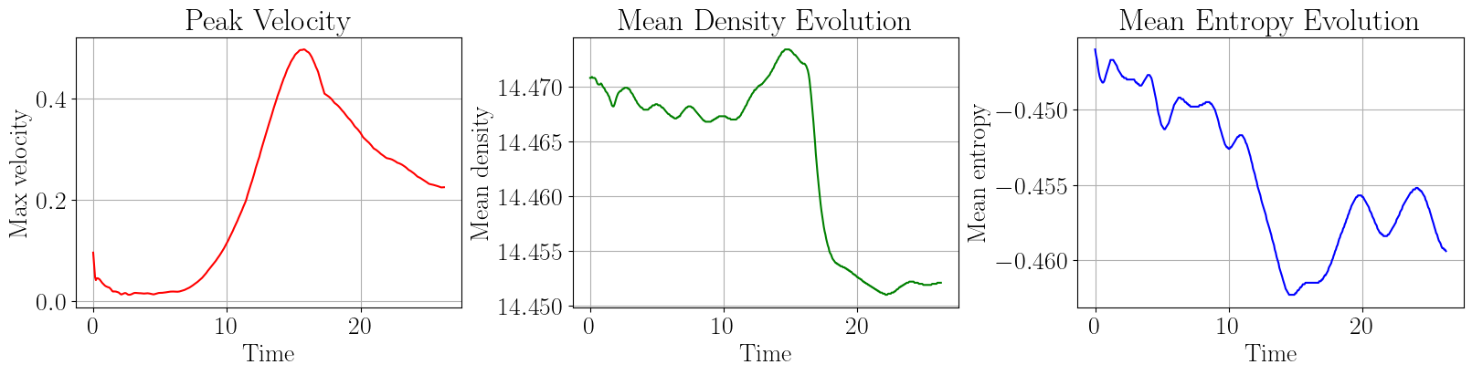
Maximum velocity and mean density and entropy.

You can download the python script inside the corresponding python folder: conv-slab/python/vmax_meanrho_means.py

Timestep diagnostics - Monitoring numerical stability:

# Check timestep limitations to ensure numerical stability
# Create simulation object
sim = pc.sim.simulation(sdir)

# Read time series
ts = pc.read.ts(sim=sim)

# Select the number of rows and columns
rows = 1
cols = 1

# Create figure
fig, axs = plt.subplots(nrows=rows, ncols=cols, figsize=(12, 6), constrained_layout = True)

# Plot maximum velocity to see if the flow is becoming turbulent
axs.plot(ts.t, ts.dtc, label='dtc (compressibility)',ls='--', linewidth=2)
axs.plot(ts.t, ts.dtu, label='dtu (velocity)',ls='-.', linewidth=2)
axs.plot(ts.t, ts.dtnu, label='dtnu (viscosity)',ls=':', linewidth=2)
axs.plot(ts.t, ts.dtchi, label='dtchi (heat conduction)', ls='-',linewidth=2)
axs
axs.set_xlabel('Time')
axs.set_ylabel('Timestep constraint')
axs.set_title('Timestep Limiting Factors')
fig.legend(loc='upper right',bbox_to_anchor=(1, 0.8))
axs.grid(True)

plt.show()

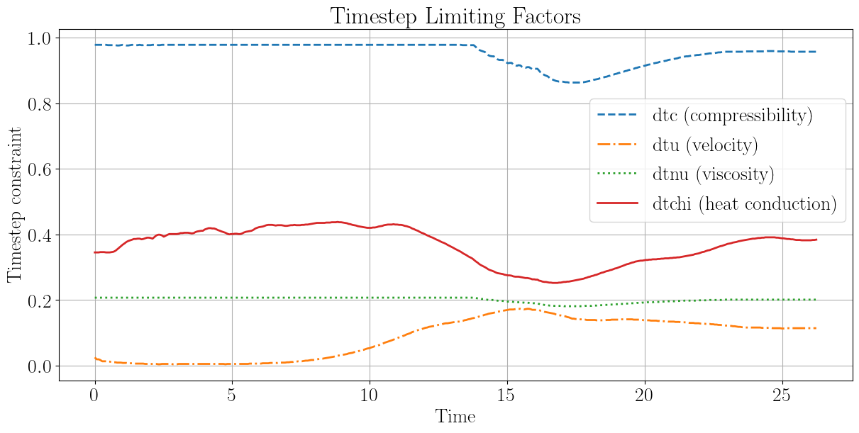
You can download the python script inside the corresponding python folder: conv-slab/python/pstability.py

Reading snapshot data for field visualization:

Unlike full 3D snapshots (var files), slices provide 2D cross-sections of the domain at specific locations. This is memory-efficient and sufficient for visualizing convective structures. Before reading the slices, they must be assembled from video files:

# Compile the reader
pc_build read_all_videofiles
# Assemble the slices
./src/read_all_videofiles.x

Repeat this every time the simulation evolves and new timesteps are generated.

The slices contain the following structure: slices.plane.field, with planes xy (horizontal), xz and yz (vertical), and fields uu1 (ux), uu2 (uy), uu3 (uz), and lnrho. Each slice has shape (nt, nx, ny) or equivalent for vertical planes.

Real-time interactive visualization with animate_interactive:

For quick monitoring during simulation runs, the pc.visu.animate_interactive function provides an efficient way to visualize time-evolving slices without generating static plots. This is ideal for understanding convective dynamics as they develop. By examining both horizontal and vertical slices, you gain a complete 3D perspective of the convection.

Horizontal slices (top view):

import pencil as pc
import numpy as np

# Read slices
slices = pc.read.slices()

# Get horizontal (xy) slice at the top of the domain
# uu3 is the vertical velocity component (uz)
uuz_xy = slices.xy.uu3

# Get density at the top
lnrho_xy = slices.xy.lnrho
rho_xy = np.exp(lnrho_xy)

# z-component of the velocity at the surface
pc.visu.animate_interactive(uuz_xy, slices.xy.t, title='Vertical Velocity (uz) - Horizontal Slice')

# Density at the surface
pc.visu.animate_interactive(rho_xy, slices.xy.t, title='Density (ρ) - Horizontal Slice')

The interactive animation allows you to step through timesteps manually, observing how convective plumes (bright and dark regions of vertical velocity) rise from the superadiabatic layer and reach the upper boundary. The density visualization reveals the density perturbations associated with these plumes, showing how rising hot material is less dense and sinking cool material is denser—the hallmark of convective transport.

Vertical slices (side view):

# Read vertical slices
lnrho_xz = slices.xz.lnrho
rho_xz = np.exp(lnrho_xz)
uux_xz = slices.xz.uu1  # horizontal velocity (ux)
uuz_xz = slices.xz.uu3  # vertical velocity (uz)

# Horizontal component of velocity (shows shear and lateral flow)
pc.visu.animate_interactive(uux_xz, slices.xz.t, x_label='x', y_label='z', title='Horizontal Velocity (ux) - Vertical Slice')

# Vertical component of velocity (shows rising and sinking motions)
pc.visu.animate_interactive(uuz_xz, slices.xz.t, x_label='x', y_label='z', title='Vertical Velocity (uz) - Vertical Slice')

# Density profile showing stratification
pc.visu.animate_interactive(rho_xz, slices.xz.t, x_label='x', y_label='z', title='Density (ρ) - Vertical Slice')

The vertical perspective is crucial for understanding the stratification. The density slice reveals the superadiabatic layer (bottom, where convection is driven) and how plumes penetrate upward. The vertical velocity in this view shows the characteristic rising (positive uz) and sinking (negative uz) flows that transport energy. The horizontal velocity component demonstrates the lateral circulation patterns that develop as the convection organizes into coherent structures.

Post-processing with Python

Deriving the Rayleigh Number

The Rayleigh number is a dimensionless quantity that characterizes the strength of convection and is not specified as an input parameter but rather derived from the simulation setup. It determines whether convection will be laminar, transitional, or turbulent.

The Rayleigh number is defined as:

(1)\[Ra = \frac{g \alpha \Delta T L^3}{\nu \chi},\]

where:

\(g\) is gravitational acceleration
\(\alpha\) is the thermal expansion coefficient (for ideal gas: \(\alpha = 1/T\))
\(\Delta T\) is the temperature difference driving convection (superadiabatic excess)
\(L\) is the characteristic length scale (domain height)
\(\nu\) is kinematic viscosity
\(\chi\) is thermal diffusivity

For this setup, using parameters from run.in and start.in:

Gravity: \(g = 1\) (normalized units)
Viscosity: \(\nu = 4 \times 10^{-3}\)
Thermal conductivity: \(K = 8 \times 10^{-3}\) → thermal diffusivity \(\chi \approx 3.2 \times 10^{-3}\)
Domain height: \(L = 2\)
Temperature (from \(c_s^2 = \gamma T\)): \(T_0 \approx 0.2\) → \(\alpha = 1/T_0 = 5\)
Superadiabatic excess (from polytropic indices \(m_{\text{poly},0}=1\) and \(m_{\text{poly},1}=3\)): \(\Delta T \approx 0.4\)

Result: \(Ra \approx 1.25 \times 10^6 \approx 10^{6.1}\)

This is a high Rayleigh number in the turbulent regime. The long simulation duration (4000 timesteps with \(\Delta t_{\text{code}} \sim 0.001\)) allows the system to develop complex time-dependent flows and turbulent structures, making this an excellent case for studying developed convective turbulence.

To compute the Rayleigh number programmatically from simulation data:

import pencil as pc
import numpy as np

# Load simulation parameters
sim = pc.sim.simulation(sdir)
p = sim.param

# Extract parameters
g = np.abs(p.gravz)  # gravitational acceleration
nu = p.nu  # kinematic viscosity
hcond0 = p.hcond0  # thermal conductivity coefficient
gamma = p.gamma  # heat capacity ratio
cs0 = p.cs0  # reference sound speed
rho0 = p.rho0  # reference density
Lz = p.Lxyz[2]  # domain height

# Compute derived quantities
T0 = cs0**2 / gamma  # reference temperature
alpha = 1.0 / T0  # thermal expansion coefficient
cp = gamma / (gamma - 1.0)  # specific heat at constant pressure
chi = hcond0 / (rho0 * cp)  # thermal diffusivity

# Estimate superadiabatic excess from polytropic indices
dT = (p.mpoly1 - p.mpoly0) * cs0**2 / gamma

# Compute Rayleigh number
Ra = (g * alpha * dT * Lz**3) / (nu * chi)

print(f"Rayleigh number: Ra = {Ra:.2e}")
print(f"Convection regime: {'Laminar (Ra < 1e3)' if Ra < 1e3 else 'Transitional (1e3 < Ra < 1e6)' if Ra < 1e6 else 'Turbulent (Ra > 1e6)'}")

Analysis Scripts

The simulation results can be analyzed and visualized using Python scripts that leverage the Pencil Code Python library. Two key analysis scripts are provided: thermo.py for thermodynamic stratification and pc_flux.py for energy flux analysis.

Initial Thermodynamic Variables

Script: thermo.py

The thermo.py script reads the simulation parameters and computes the initial stratification profiles for temperature, density (lnrho), and entropy. This provides insight into the background state that drives convection.

Usage:

python thermo.py

Output:

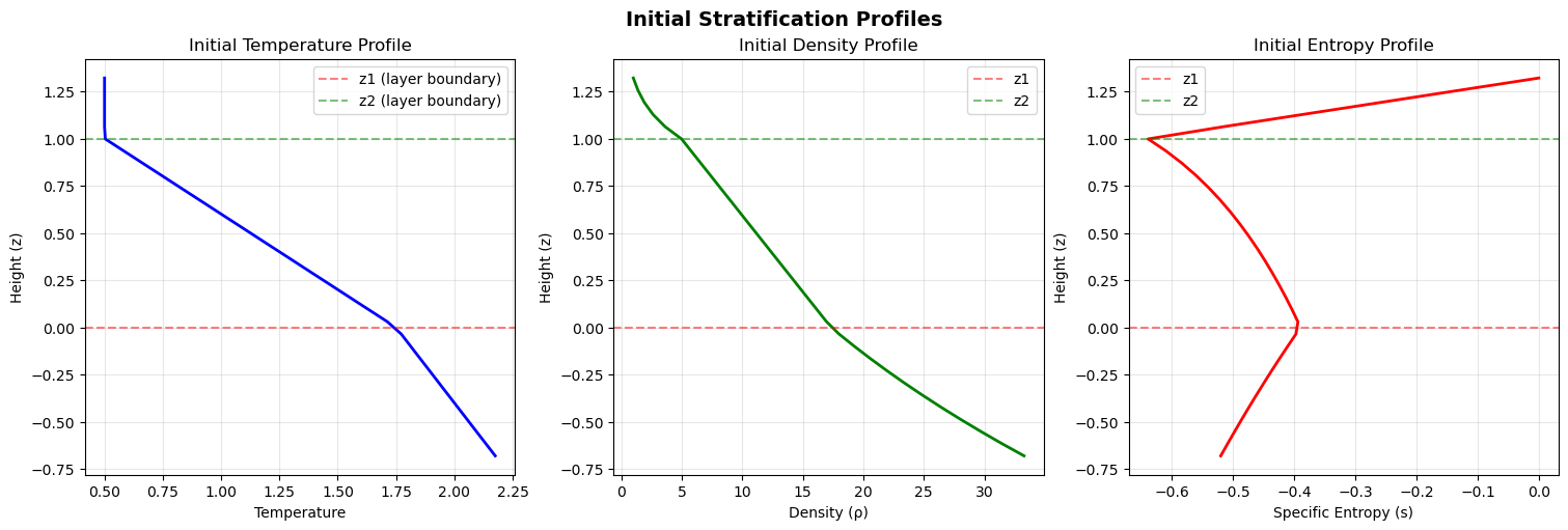
The three-panel figure shows:

Left panel (Temperature T): The temperature profile exhibits the characteristic superadiabatic layer at the bottom (increasing temperature with height) where convection is driven. Above this unstable region is a stable layer where temperature decreases with height.
Middle panel (Density ln(ρ)): The logarithmic density profile shows how the fluid density decreases with height due to hydrostatic equilibrium. The density gradient is steepest in the lower layers, reflecting the strong compression at depth.
Right panel (Entropy s): The entropy profile shows the superadiabatic gradient—entropy increases with height in the lower layer, creating the unstable stratification that triggers convection. The entropy profile is crucial for understanding the convective instability.

Design: This script uses the Pencil Code Python library to read simulation parameters via sim.param (accessing cached parameter dictionary) and computes polytropic stratification using the equations of state. It demonstrates best practices for parameter access and function-based visualization in Python analysis scripts.

Energy Flux Analysis and Visualization

Script: pc_flux.py

The pc_flux.py script reads xy-averaged data from the simulation and analyzes the vertical profiles of energy fluxes. These fluxes represent different mechanisms of energy transport in the convective layer.

Usage:

python pc_flux.py

The script computes and visualizes six flux components:

Kinetic energy flux (fkin): Energy transported by bulk fluid motion
Radiative flux (frad): Energy transported by radiation
Convective flux (fconv): Energy flux due to convective plumes (enthalpy flux)
Turbulent flux (fturb): Energy flux from turbulent fluctuations (typically zero in laminar convection)
Cooling flux (fcool): Integrated radiative cooling (computed from cooling rate by vertical integration)
Total flux (ftot): Sum of all flux components (should approach constant with height for steady energy balance)

Output Figures:

Final time flux profiles:

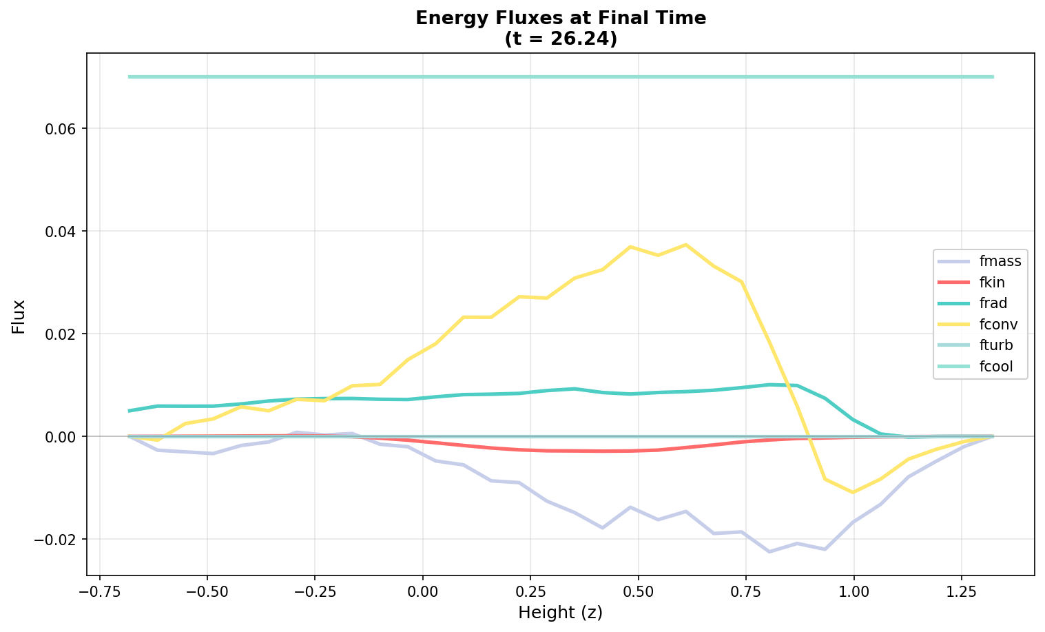
This figure shows all flux components as vertical profiles at the final timestep. It reveals the instantaneous energy transport mechanisms:

The convective flux (fconv) is the dominant transport mechanism, with peak values around 0.037 in the interior. This is expected in a Rayleigh-Bénard convection regime where buoyancy-driven plumes are the primary energy transport.
The kinetic energy flux (fkin) shows small variations with depth, reaching extremes around -0.003. The negative values indicate energy flowing downward in some layers.
The radiative flux (frad) is relatively small (±0.01), but plays an important role around the z2 boundary layer region where cooling is applied.
The cooling flux (fcool) is strictly non-negative (cooling always removes energy) with a value of 0.07 throughtout

Flux evolution over time:

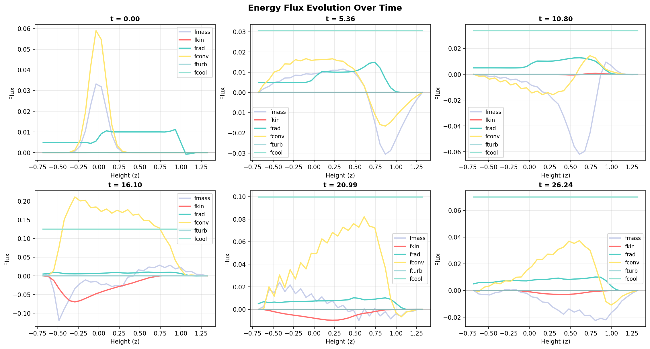
This six-panel figure shows how each flux component evolves with depth and time. Each panel displays flux profiles at several timesteps (colored curves), revealing temporal variations:

fmass (red): The distribution of mass changes with time at the different heigths.
fkin (blue): Shows temporal variability with oscillations indicating dynamic convective activity.
frad (green): Small but non-zero values, with slight temporal variations as the radiation field adjusts.
fconv (orange): The dominant and most variable flux component, showing how convective transport changes as the flow organizes.
fturb (violet): Remains at zero, confirming the flow is still laminar (no developed turbulence).
fcool (teal): Shows evolution of the cooling profile with time, always non-negative.

Total flux time series:

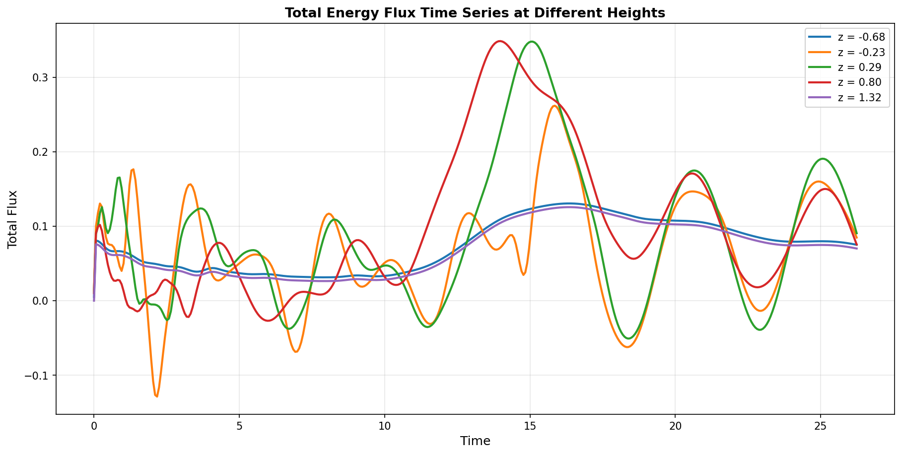
This figure shows how the total energy flux evolves with time at different heights in the domain:

Each curve represents the total flux (sum of all components) at a fixed height
The horizontal dashed line at constant flux indicates perfect energy balance (steady state energy transport)
The temporal variations in total flux reveal how the system adjusts toward a steady state
Top layers (near cooling region): Show larger total flux due to the imposed cooling
Middle layers: Exhibit relatively stable total flux as convection maintains quasi-steady energy transport
Bottom layers: Show variability as the convection develops from initial perturbations

Flux Statistics Summary:

The analysis of xy-averaged flux data reveals the dominant energy transport mechanisms:

fmass (Mass flux):
  Min: -1.578720e-01    Max: 1.007140e-01    Mean: -1.047720e-02
  At final time - Min: 0.0, Max: 0.0 (confirms mass conservation)

fkin (Kinetic energy flux):
  Min: -7.157110e-02    Max: 7.051480e-03    Mean: -4.357272e-03
  At final time - Min: 0.0, Max: 0.0
  → Net downward kinetic energy transport on average

frad (Radiative flux):
  Min: -7.813110e-04    Max: 1.522690e-02    Mean: 6.529695e-03
  At final time - Min: -1.802000e-04, Max: 1.501410e-04
  → Small but non-zero; slightly upward on average

fconv (Convective flux):
  Min: -1.200630e-01    Max: 2.765830e-01    Mean: 2.039807e-02
  At final time - Min: 0.0, Max: 0.0
  → Dominant transport mechanism; mean upward heat transport

fturb (Turbulent flux):
  Min: 0.0    Max: 0.0    Mean: 0.0
  At final time - Min: 0.0, Max: 0.0
  → Zero throughout; flow remains laminar

fcool (Cooling flux):
  Min: 0.0    Max: 1.255281e-01    Mean: 7.020112e-02
  At final time - Min: 0.0, Max: 1.255281e-01
  → Always non-negative; cooling enforced in upper layers

Physical Interpretation:

Energy Balance: The total energy flux (fconv + frad + fcool + fkin) should approach a constant value with height at steady state, indicating energy conservation. The variations shown in the time series reflect the system’s evolution toward this balance.
Convective Dominance: The convective flux (fconv) with mean value 0.0204 is the primary energy transport mechanism, as expected for Rayleigh-Bénard convection. Its maximum (~0.276) significantly exceeds other components, confirming that buoyancy-driven plumes transport most of the energy.
Kinetic Energy Sink: The mean kinetic energy flux is slightly negative (-0.00436), indicating that on average, kinetic energy dissipates downward in the domain. This energy is ultimately dissipated through viscosity.
Radiative Cooling: The cooling flux (fcool) with mean value 0.0702 represents the imposed radiative cooling in the upper boundary layer. At the final time, this cooling concentrates at the surface (max = 0.1253), maintaining the superadiabatic stratification.
Turbulence Absence: The zero turbulent flux confirms that the simulation remains in a laminar convective regime. Higher Rayleigh numbers or longer simulation times would eventually lead to turbulent fluctuations.

Design: The pc_flux.py script demonstrates efficient use of xy-averaged data through the pc.read.aver() function. It includes three separate visualization functions (plot_fluxes_final_time, plot_fluxes_time_evolution, plot_total_flux_time_series) that can be called independently, following best practices for modular and reusable code in scientific computing.

Acknowledgments

This tutorial has been written with the aid of GitHub Copilot.